MCB128: AI in Molecular Biology (Spring 2026)
(Under construction)
(Now hiring TFs Fall 2026)
- A single neuron
- Parts of a single neuron (perceptron)
- The space of weights
- What can a single neuron learn? to be a binary classifier
- The learning rule
- The error function
- Backpropagation
- The batch gradient descent learning algorithm for a feedforward network
- The on-line stochastic gradient descent learning algorithm
- How well does the batch learning algorithm do?
- Regularization: beyond descent on the error function
- What does a perceptron cannot do?
- RNA Functional Classification using a perceptron
block 0:
A single neuron / DNA Functional Classification
In this lecture, I follow David Mackay very closely. In particular his lectures 15 and 16, which correspond to Chapters 39, 41 and 42 of his book Information Theory, Inference, and Learning algorithms.
A good reference for the basics of deep learning is this book (pdf attached) Understanding DL. I strongly recommend it.
The original perceptron dates back to Frank Rosenblatt’s paper “The perceptron: a probabilistic model for information storage and organization in the brain” from 1958.
As a practical implementation of a simple perceptron in molecular biology, we will study the work “Use of the ‘Perceptron’ algorithm to distinguish translational initiation sites in E. coli” “, by Stormo et al. (1986) in which they use a perceptron to identify translation initiation sites in E.coli.
A single neuron
Here is the code associated to this section
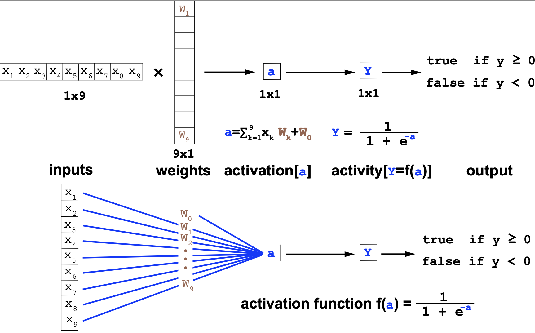
A single neuron or perceptron (Figure 1) has
- The inputs \(\mathbf{x}=(x_1,\ldots,x_I)\),
- Parameters \(\mathbf{w}=(w_1,\ldots,w_I)\), usually called the weights.
- One output \(y\) which is also called the activity,
The neuron adds up the weighted sum of the inputs into a variable called the activation \(a\),
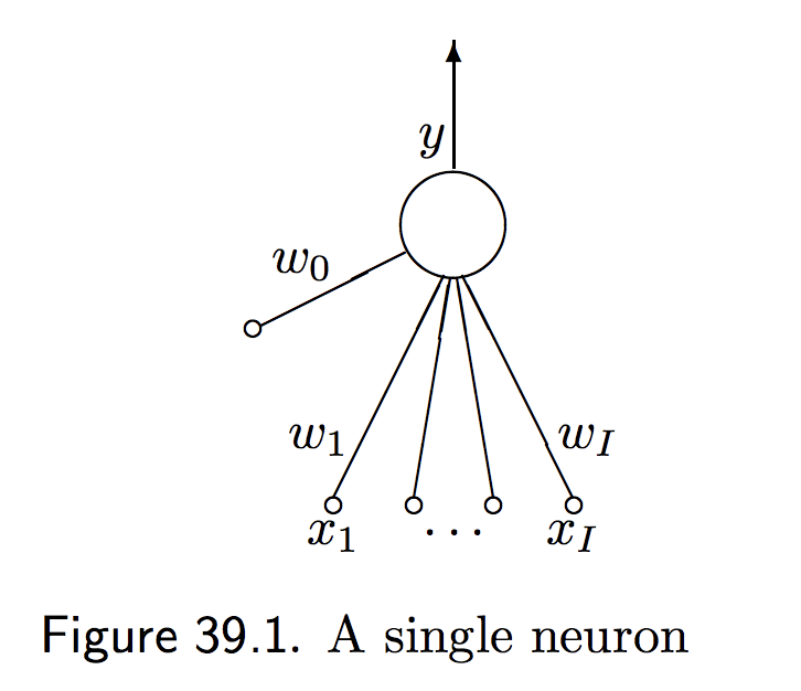
Figure 1. One neuron (from D. Mackay's chapter 39).
where \(w_0\) called the bias is the activation in the absence of inputs.
The activity of the neuron \(y\) is a function of the activation function \(f(a)=y\). Several commonly used forms for the activity are
-
The linear logistic function
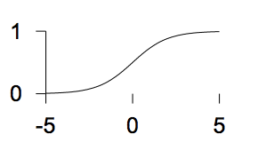 \(f(a) = \frac{1}{1+e^{-a}}\)
 -
The sigmoid (tanh) function
 \(f(a) = tanh(a)\)
 -
The step function
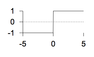 \(f(a) = \left\{
\begin{matrix}
1& a > 0\\
0& a \leq 0
\end{matrix}
\right.\)
\(f(a) = \left\{
\begin{matrix}
1& a > 0\\
0& a \leq 0
\end{matrix}
\right.\)
Depending in how we combine many single neurons, there is essentially two types of networks: feedforward networks, where all the information flows in one direction, and feedback networks where all nodes are connected (Figure 2).
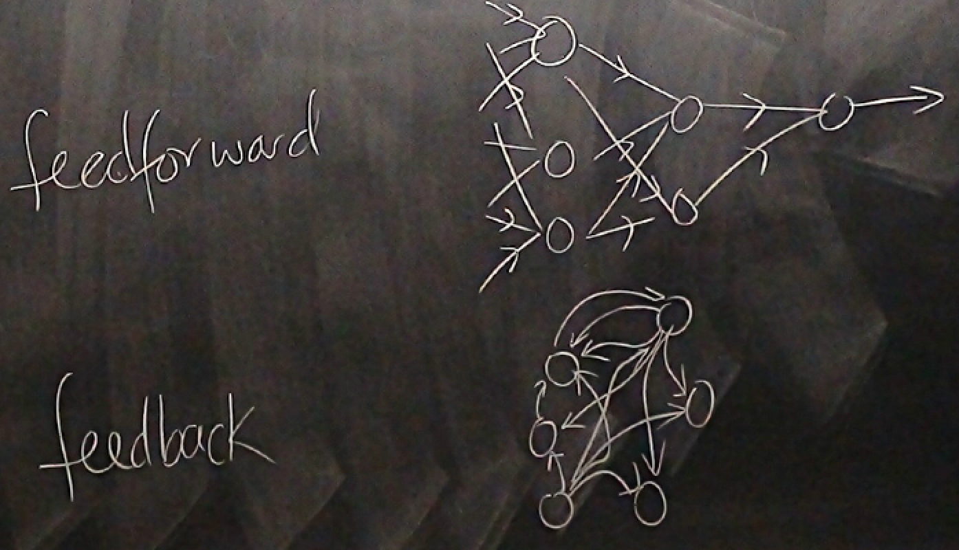
Figure 2. Two type of networks (from D. Mackay's Lecture 15).
Parts of a single neuron (perceptron)
As a recap, the basic concepts of a neuron are
-
The Architecture. A single neuron has a number \(I\) of inputs \(x_i\), and one output \(y\). Each input has associated a weight \(w_i\), for \(0\leq i \leq I\).
-
The Activation. In response to the inputs, the neuron computes the activation
and \(x_0=1\), so we can add the bias in the same equation.
-
The Activity rule. The neuron output, \(y(\mathbf{x},\mathbf{w})\), is set as a logistic/step function of the activation and the inputs \(\mathbf{x}\).
We are going to study a neuron in which the output is between (0,1), such that the activity \(y(\mathbf{x},\mathbf{w})\) is given by the logistic function
\[y(\mathbf{x},\mathbf{w}) = \frac{1}{1+e^{-a}} = \frac{1}{1+e^{-\mathbf{w}\cdot \mathbf{x}}}.\]The activity \(0\leq y(\mathbf{w},\mathbf{x})\leq 1\) can be seen as the probability according to the neuron that the input deserves a response, and the neuron fires (\(y=1\)) or that the input is not worth a response and the neuron does not fire (\(y=0\)).

Figure 3. Neuron activity for a neuron with two inputs as a function of the inputs. The values of the weights are: w0 = +15, w1 = -2 w2 = -1. We use the logistic function to describe the activity of the neuron.
The space of weights
Consider the simple situation of only two input to the neuron \(\mathbf{x}=(x_1, x_2)\), and only two weights \(\mathbf{w}=(w_1, w_2)\) and no bias. The neuron’s activation is given by
\[y = \frac{1}{1+ e^{-(w_0 + w_1 x_1 + w_2 x_2)}}\]and we can plot it as a function of the inputs as in Figure 3.
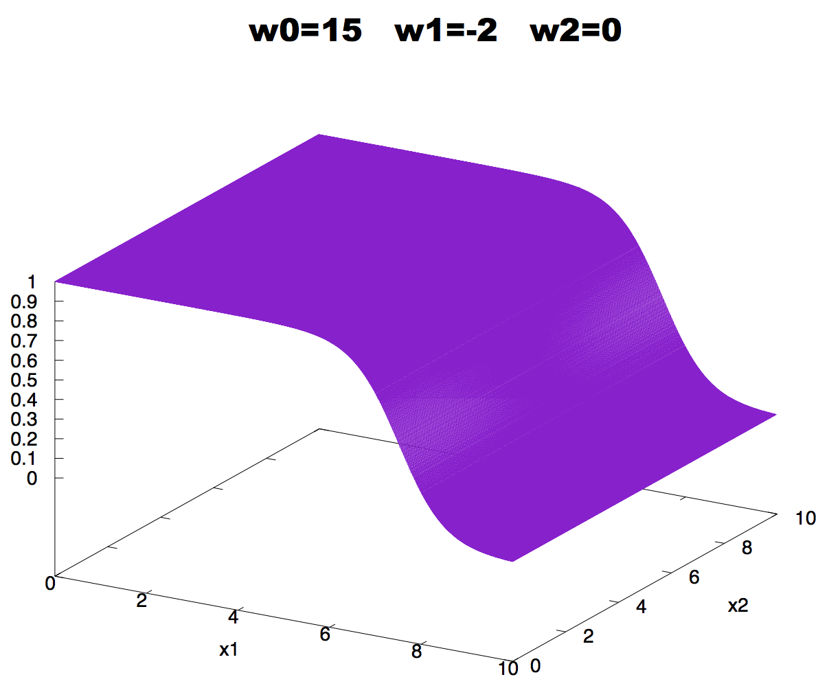
Figure 4. Effect on neuron activity of a zero weight.
If a weight is zero, there is no activity change associated with changes in the corresponding input, as described in Figure 4.
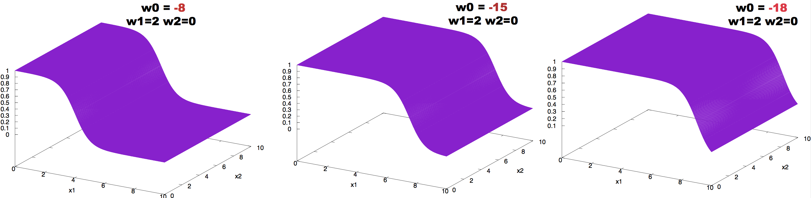
Figure 5. Effect on neuron activity of the bias term.
The effect of changing the value of the bias can be observed in Figure 5.
The effect of changing the value of the weights can be observed in Figure 6.
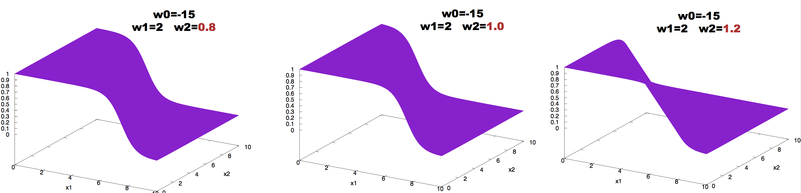
Figure 6. Effect on neuron activity of changes in one of the weights.
We can also use contour plots, in which we represent in the inputs space lines corresponding to different values of the activity \(y\). Using contour plots we observe in Figure 7 the effect of making the weight larger or smaller in absolute magnitude. Doubling the weights makes the contour lines closer to each other, while halving the weight make the same contour lines wider.
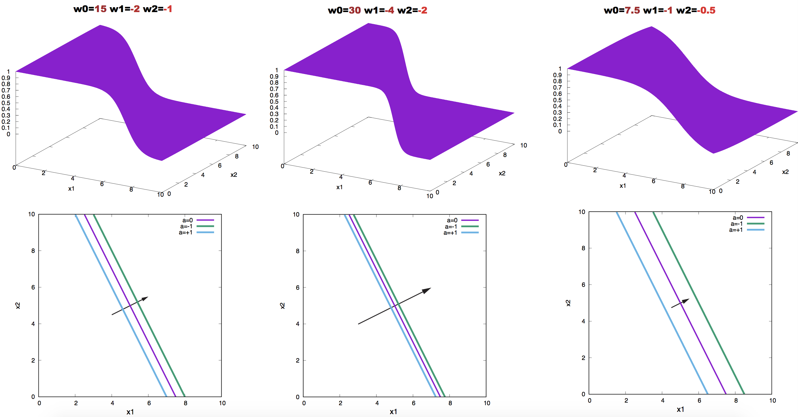
Figure 7. Effect on neuron activity of scaling the weights. The contours correspond to the values a = 0.0, 1, and -1. Arrows point in the direction of the weight vector.
What can a single neuron learn? to be a binary classifier
Imagine that you want to separate apples from oranges from a bucket in which they are all mixed up. Would you trust a single neuron to do that?
The data given in Figure 9 is a collection of 5 apples and 5 oranges, for which we have two types of data (two inputs): color and roughness.
The learning rule
The central idea of supervised learning is this: given a number of examples of the input vector \(\mathbf{x}^{(1)}\ldots \mathbf{x}^{(N)}\) and their target output \(t^{(1)}\ldots t^{(N)}\), we hope the neuron will learn their relationship (whichever that is).
Training the network requires finding the values of the weights that best fit the training data. If the neuron is well trained, given an input \(\mathbf{x}\) will produce an output \(y\) which is very close to the target \(t\).
Data: \(D = \{\mathbf{x}^{(1)}, t^{(1)},\ldots, \mathbf{x}^{(N)}, t^{(N)}\}\)
Outputs: \(\{y^{(1)},\ldots, y^{(N)}\}\)
Error: \(\{y^{(1)}-t^{(1)},\ldots,y^{(N)}-t^{(N)}\}\) where we expect these errors to be small.
Thus “learning” is equivalent to adjusting the parameters (weights) of the network such that the output \(y^{(n)}\) of the network is close to the target \(t^{(n)}\) for all \(n\) examples.
In our apples and oranges example, let’s give an assignment of \(t=1\) for an apple, and \(t=0\) for an orange. A well trained neuron will produce assignments \(y\) similar to these:
Orange_1:  y(Orange_1, w) = 0.01
Orange_2:  y(Orange_2, w) = 0.09
Orange_3:  y(Orange_3, w) = 0.05 ...

Apple_1   y(Apple_1,  w) = 0.91
Apple_2   y(Apple_2,  w) = 0.97
Apple_3   y(Apple_3,  w) = 0.99...
How to do that? We find a function to optimize.
The error function
For each input \(\{\mathbf{x}^{(n)}, t^{(n)}\}\), we introduce an objective function that will measure how close the neuron output \(y(\mathbf{x}^{(n)},\mathbf{w})\) is to \(t^{(n)}\). That objective function is also called the error function.
We introduce the error function (or loss function)
\[G(\mathbf{w}) = - \sum_{n=1}^{N} \left[ t^{(n)} \log(y^{(n)}) + (1-t^{(n)}) \log(1-y^{(n)})\right],\]where \(y^{(n)} = y(\mathbf{x}^{(n)},\mathbf{w})\).
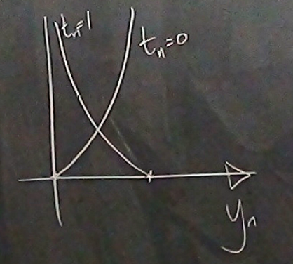
Figure 8. Contribution to the error function G(w) for one data point as a function of y(n) for the two possible cases t(n)=0 and t(n)=1. (From D. Mackay's video lecture 15.)
For each data point \((\mathbf{x}^{(n)},t^{(n)})\), its contribution to the error function is given by Figure 8.
As a binary classification problem, such as sorting apples from oranges, we can interpret \(y(\mathbf{x},\mathbf{w})\) and \(1-y(\mathbf{x},\mathbf{w})\) (both between zero and one) as the probabilities of the two possible events: apple (\(t=1\)) or orange (\(t=0\)) for an input \(\mathbf{x}\) given the weights of the neuron.
\[y^{(n)} = (y(\mathbf{x}^{(n)},\mathbf{w}), 1-y(\mathbf{x}^{(n)},\mathbf{w})).\]The labels can also be expressed as a discrete probability distribution,
\[t^{(n)} = (t^{(n)}, 1-t^{(n)})\]Then the error \(G(\mathbf{w})\) is the sum to all data points in the training set of the cross entropy between the labels \(\{t^{(1)},\ldots,t^{(N)}\}\) and the outputs \(\{y^{(1)},\ldots,y^{(N)}\}\).
Backpropagation
The training process is an exercise of minimizing \(G(\mathbf{w})\), that is, of adjusting the weights so that \(G(\mathbf{w})\) reaches it lowest value.
Notice that \(G(\mathbf{w})\) is bound by below by zero,
\[G(\mathbf{w}) \geq 0,\]and it is zero only when \(y^{(n)}(\mathbf{x},\mathbf{w}) = t^{(n)}\).
To minimize, we take the derivative of \(G(\mathbf{w})\) respect to one of the weights \(w_i\) given by
\[\frac{\delta G(\mathbf{w})}{\delta w_i} = -\sum_n \left[\frac{t^{(n)}}{y^{(n)}}-\frac{1-t^{(n)}}{1-y^{(n)}}\right]\, \frac{\delta y^{(n)}}{\delta w_i} = -\sum_n \frac{t^{(n)}-y^{(n)}}{y^{(n)} (1-y^{(n)})}\, \frac{\delta y^{(n)}}{\delta w_i}\]Introducing
\[\frac{\delta y^{(n)}}{\delta w_i} = x^{(n)}_i\, \frac{e^{-\mathbf{w}\mathbf{x}^{(n)}}}{(1+e^{-\mathbf{w}\mathbf{x}^{(n)}})^2} = x^{(n)}_i y^{(n)} (1-y^{(n)}),\]we obtain,
\[\frac{\delta G(\mathbf{w})}{\delta w_i} = -\sum_n \left[t^{(n)}-y^{(n)}\right] x^{(n)}_i.\]Taking all derivative together we construct the gradient vector,
\[\mathbf{g} = \frac{\delta G(\mathbf{w})}{\delta \mathbf{w}} = -\sum_n \left[t^{(n)}-y^{(n)}\right] \mathbf{x}^{(n)}.\]The quantity \(e^{(n)} = t^{(n)}-y^{(n)}\) is referred to as the error.
Backpropagation in the neural network community referees to given the errors, to calculate the gradient
\[\mathbf{g} = \sum_n -e^{(n)}\,\mathbf{x}^{(n)}.\]Backpropagation \(\longleftrightarrow\) differentiation.
Then we can implement a “gradient descent” method in which we iteratively update the weights by a quantity \(\eta\) in the opposite direction to the gradient,
\[\mathbf{w}^{new} = \mathbf{w}^{0ld} - \eta\,\mathbf{g} = \mathbf{w}^{0ld} + \eta\,\sum_n e^{(n)}\,\mathbf{x}^{(n)}\]The parameter \(\eta\) in the neural network community is referred to as the learning rate. And it is a free parameter that one has to set somehow.
Depending on whether we update the weights by looking to all data point at the time, or each one of them independently, we can distinguish two different algorithms, the batch learning algorithm and the on-line learning algorithm.
The batch gradient descent learning algorithm for a feedforward network
For a data set \(\{\mathbf{x}^{(n)}, t^{(n)}\}_{n=1}^N\),
- Start with a set of arbitrary weights \(\mathbf{w}_0\), and use the activity rule to calculate for each data point
- Use backpropagation to calculate the next set of values for the weights \(\mathbf{w}_1\) as
We can repeat this two steps for a fixed and large number of iterations, or until the errors for all data points are smaller than a desired small number.
The on-line stochastic gradient descent learning algorithm
Alternative, we could update all weights, by taking one data point at the time. Start with a set of arbitrary weights \(\mathbf{w}_0\)
- Select one data point \(m\in [1,N]\), and use the activity rule to calculate
- Use backpropagation to calculate the next set of values for the weights \(\mathbf{w}_1\) as
Then one can go back to select another point from the data set and repeat the process.
While batch learning is a gradient descent algorithm, on-line learning algorithm is a stochastic gradient descent algorithm.
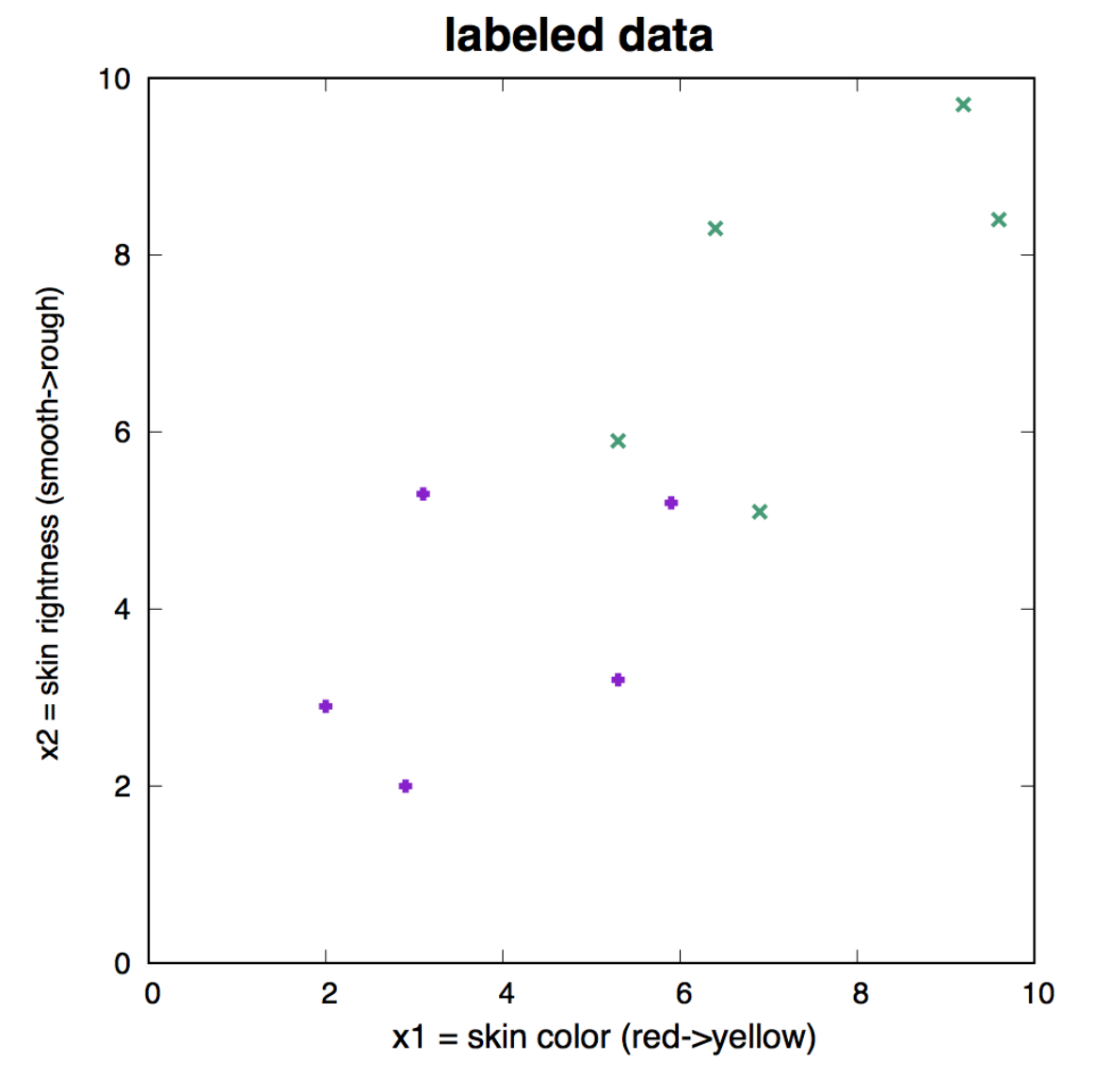
Figure 9. Labeled data that we use as training set to learn the three weights of the neuron. Apples are represented in purple, and have target value t=1. Oranges are represented in green, and have target value t=0.
How well does the batch learning algorithm do?
Let’s go back to our apple/oranges classification task, using a neuron with two inputs \(x_1\) and \(x_2\). Perhaps \(x_1\) could be a measure of the skin color of the fruit, and \(x_2\) could be a measure of the roughness of the skin for each fruit example.
There are then three weights \(w_0, w_1, w_2\), including the bias \(w_0\). The activity rule is given by
\[y(\mathbf{w},\mathbf{x}) =\frac{1}{1+e^{-(w_0+w_1 x_1 + w_2 x_2)}}.\]
Figure 10. Parameter evolution as a function of the number of iterations in the batch-learning algorithm.
We assume we have labeled data, that is \(N=10\) examples in which we have measured the value of the two variables \(x_1\) and \(x_2\), and we know whether they are apples, A(t=1) or oranges, O(t=0). The labeled data is given in Figure 9.
We perform batch gradient descent with learning rate \(\eta = 0.01\). Figure 10 describes the changes in the parameter values as a function of the number of iterations. Figure 11 describes contour plots for different number of iterations.
Regularization: beyond descent on the error function
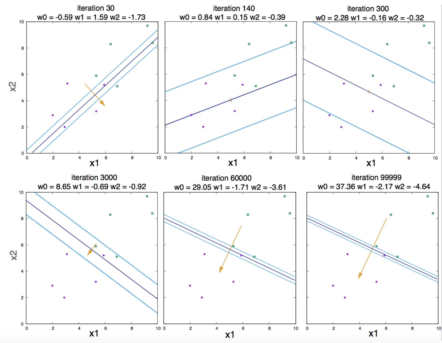
Figure 11. Contour plots for different number of iterations
We have seen that if the data is in fact linearly separable, the algorithm works. But as the number of iterations becomes larger and larger, the weights also become larger in magnitude, and the logistic function becomes steeper and steeper (Figure 11). That is an undesirable behavior named overfitting.
Why is it undesirable?
A way to avoid having weights arbitrarily large and overfitting to the data has the name of regularization. The idea consists of adding a term to the optimization function such that it penalizes large values of the weights. We introduce the modified objective function
\[M(\mathbf{w}) = G(\mathbf{w}) + \alpha R(\mathbf{w})\]where
\[R(\mathbf{w}) = \frac{1}{2}\,\sum_i w_i^2.\]The weight update rule in the presence of this regularization becomes
\[\mathbf{w}^\prime = (1-\alpha\eta)\, \mathbf{w} + \eta \sum_n\left(t^{(n)}-y^{(n)}_0\right) \mathbf{x^{(n)}},\]and the parameter \(\alpha\) is called the weight decay regularizer.
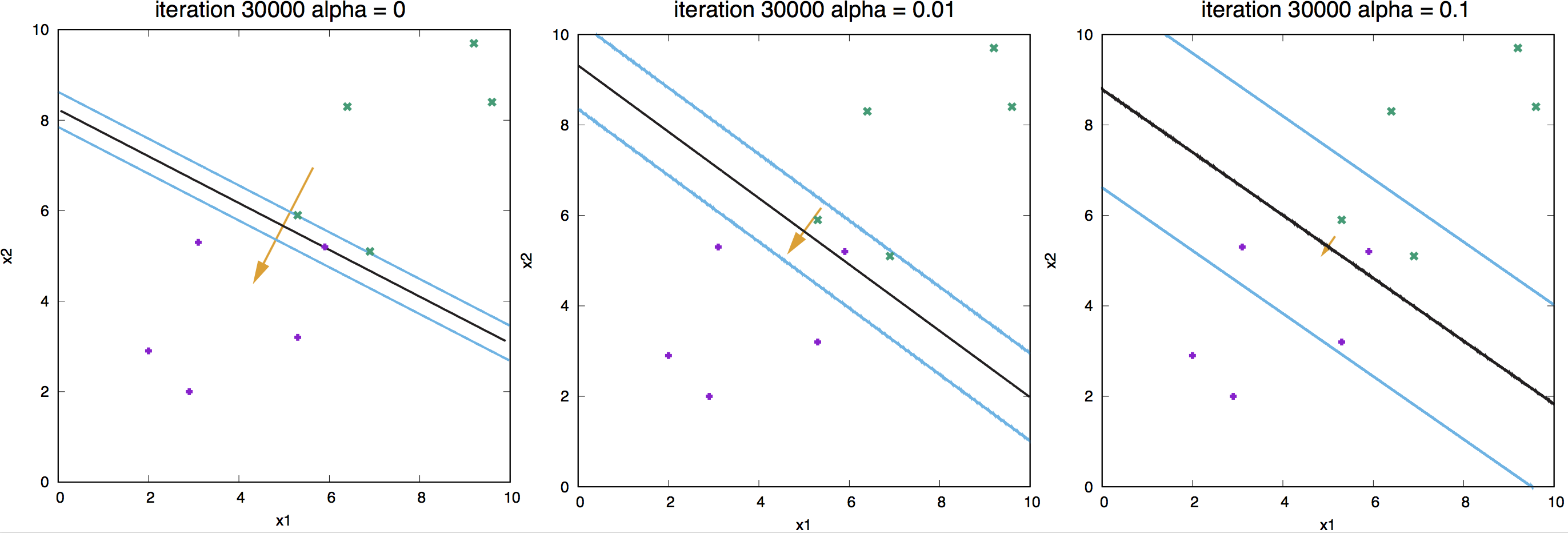
Figure 12. Effect of regularization for a linear neuron.
In Figure 12, we show examples of different weight-decay regularizer values and its effect on the learned weights.
What does a perceptron cannot do?
When the data is not linearly separable, the perceptron cannot reach a solution.
In our previous example, the set of oranges and apples were clearly separable Figure 13a, now consider another case in which the data looks like in Figure 13b. We observe that the data cannot be separated linearly, and as a results the loss function does not converge.
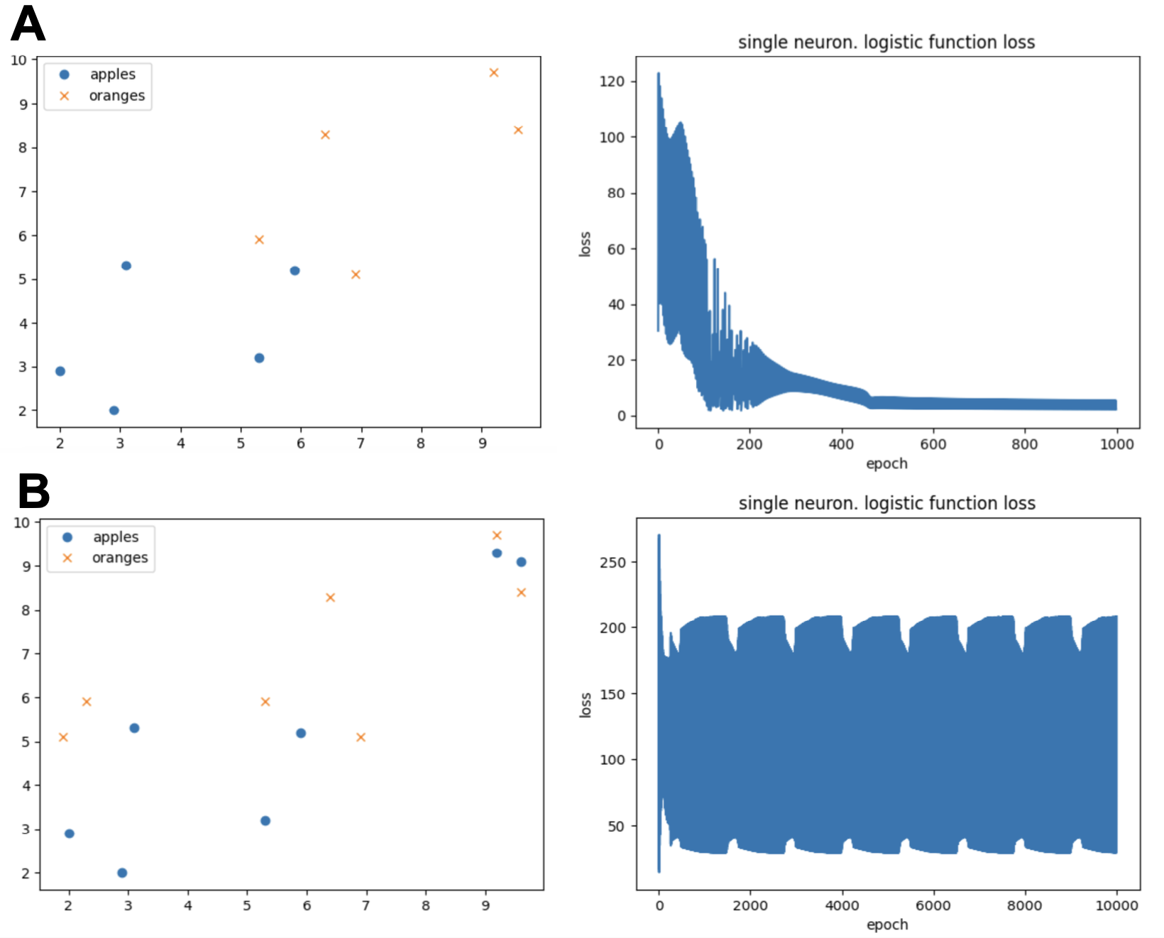
Figure 13. "The Ice Age" in Machine Learning (ML). (A) A linearly separable case. The perceptron loss indicates convergence. (B) A non-linearly separable case. The perceptron loss indicates not convergence.
This result was first described by Minsky & Papert (1969). The result halted research in neural networks for a while (the “ice age” of neural networks). The introduction of Multilayer perceptron that we will discuss next, resolved the hiatus in the 1980s.
Here is the code associated to this section. It includes a simple perceptron used to classify the example of apples and oranges. It also includes an example where the perceptron cannot classify as in Figure 13. This code also makes the generalization from binary classification to a softmax output that can be used for multi-decision classification.
RNA Functional Classification using a perceptron
Here is the code associated to this section
“Use of the ‘Perceptron’ algorithm to distinguish translational initiation sites in E. coli” (1986) is probably one of the first applications of perceptions in molecular biology.
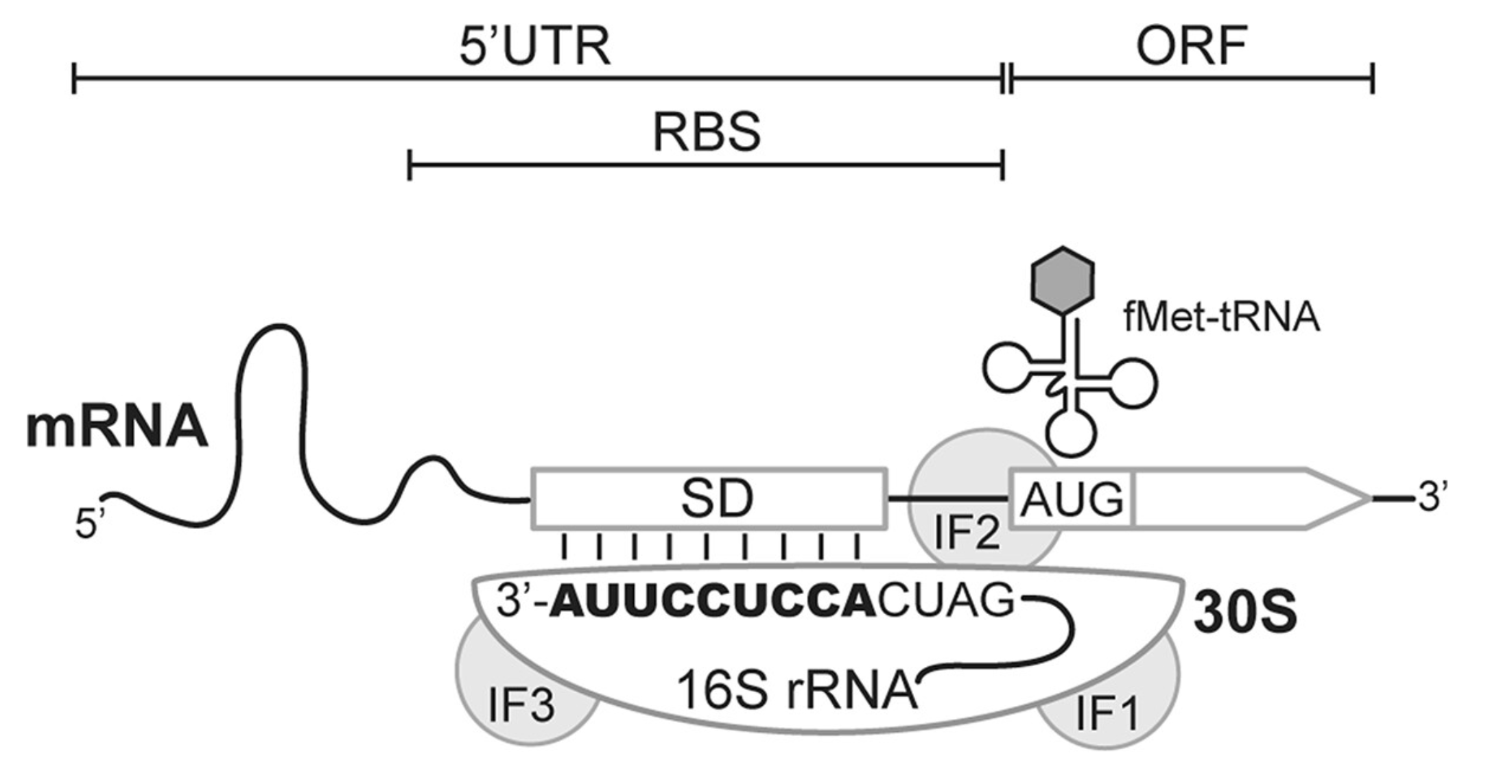
Figure 14. Translation initiation in bacteria.
In bacteria, Ribosome Binding Sites (RBS) are specific regions where translation initiates (Figure 14). Ribosome binding sites are characterized by a number of features, most importantly the start codon (AUG) and the Shine-Dalgarno sequence.
The Shine-Dalgarno sequence: (Figure 15)
-
Is located 5-10 nucleotides above the AUG.
-
Has a consensus sequence AGGAGG, but there are a lot of variations.
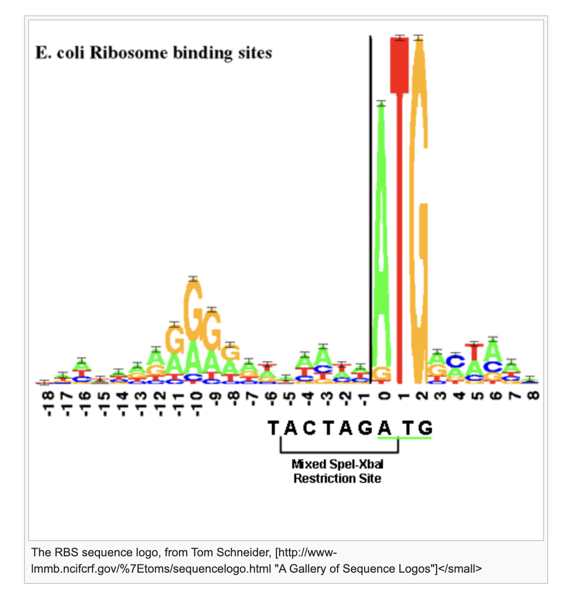
Figure 15. Consensus sequence for the Ribosome Entry Site.
The inputs
The inputs are sequences \(S\) of length \(L\). The inputs are labeled as to whether they are positive \(S^+\) or negative \(S^-\) for RBS presence. Each sequence is inputed to the perceptron using a one-hot embedding.
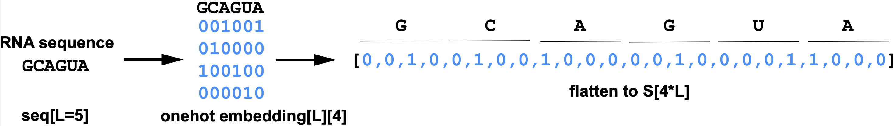
Figure 16. One-hot embedding of an RNA sequence.
The weights
This is a single neuron perceptron, thus the dimension of the weights \(W\) is the same as that of the onehot sequence, that is \(4\times L\),
Thus the product of inputs (sequence) and weights is calculated as
\[S\cdot W = \mbox{np.dot}(S,W) = \sum_{i=1} ^{i=4\times L} S_i W_i\]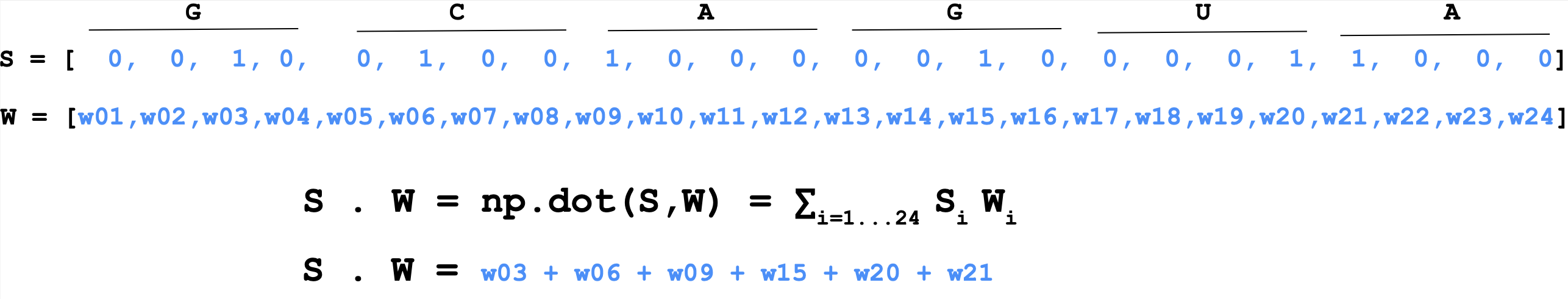 Figure 17. Product of inputs (sequence) and perceptron weights.
The Perceptron algorithm
The Stormo RBS perceptron does not use gradient descent to optimize the weight. It does not define a loss from which to backpropagate the gradients into the weight. Instead, it directly calculates the error as follows;
It defines a threshold T (set to T=0), and does the following updates
-
if \(S^+\) and \(S^+\dot W < T\), update: \(W \leftarrow W+S^+\)
-
if \(S^-\) and \(S^-\dot W > T\), update: \(W \leftarrow W-S^-\)
-
otherwise \(W\) remain unchanged
In the paper, Stormo et al. discuss the effect on discrimination due to the number of sequences (positive and negative) used to train the perceptron, and the length of sequences used in the training set. We will discuss these issues with this blocks’s homework.