MCB128: AI in Molecular Biology (Spring 2026)
(Under construction)
(Now hiring TFs Fall 2026)
- Inputs
- Outputs
- Tensors
- Models
- Model Training / Learning
- Loss/Error function
- epoch
- masking
- Gradient Descent
- Backpropagation
- The chain rule
- Vanishing gradient
- Layer Normalization
- Batch Normalization Layer
- Masking
- Adam optimization
- Forward pass
- Backward pass
- Pre-training vs Fine-tuning
- Foundational model
- Regularization
- Ablation
- overfitting
- data leakage
- Generalization
- Interpretability
- Learning
- Model Architecture
- Others
The Book of (Deep Learning) Jargon:
google machine-learning glossary
Inputs
Tokenization
Categorical variable
A variable that can take a fixed number of values. For example, DNA/RNA nucleotides can be represented as a categorical variable with four possible values A, C, G, T/U. Amino acids can be represented as a categorical variable with 21 possible values.
Embedding (or vector embedding)
An array of numbers (a vector) that represent an input. For instance, the categorical variable “RNA nucleotide” could be represented by four vectors of arbitrary dimension representing A, C, G, and U respectively.
One-hot embedding
A vector embedding representing a categorical variable such that each vector has one 1 value, and all the others are zero.
For instance, the one-hot embedding for the categorical variable “RNA nucleotide” can be given as,
A = [1,0,0,0]
C = [0,1,0,0]
G = [0,0,1,0]
U = [0,0,0,1]
Dataset
The collection of all data used to train the model. The training data usually includes the inputs for a number of examples. For some subset of the examples, we may also have labels used in [supervised training[(supervised-learning).
A dataset is usually divided into: training set, validation set and test set.
Training set
The collection of examples from the dataset that are used to train the model.
Validation set
Test set
Feature
Equivalent to inputs
Sparse Feature
A feature/input vector where most of the values are zero. For instance, the one-hot encoding is an example of a sparse feature.
Labels
First introduced in b0_lecture
Labels are associated to the examples in the training sets, and usually correspond to the categories that the neural network is trying to predict. Labels are used in all cases in which a given neural network is trained by supervised learning
Labels are different from inputs. For instance, in the case of separating apples and oranges, each of the examples is given a label \(t\), as to whether it is an apple (\(t=1\)) or an orange (\(t=0\)). For this example the inputs are the color of the fruit and the roughness of its skin.
For the Ribosomal Entry Sites perceptron, the inputs/features are the nucleotides of a RNA sequence, and each example RNA sequence is given a label \(+\) for being a ribosomal binding site (RBS) or \(-\) otherwise.
Labeled data
Labeled data is data for which in addition to consisting of the inputs (or features) for a number of examples, it also provides for each example label values of what the neural network is trying in infer. These labels become the ground truth used in supervised training to guide the optimization of the weights.
Unlabeled data
Unlabeled data is data that does not include any labels. Like in our apple/oranges data from b0, Figure 9, it would mean getting for all fruit examples all the input values for “color” and “skin roughness” without telling us whether the fruit is an apple or an orange.
Unlabeled data can be used as test
Batch (or mini-batch)
First introduced in b1_lecture. The set of data examples used in one parameter optimization step during training.
A set of minibatch optimization steps that include all the examples in the training set constitutes an epoch. The batch size is usually smaller than that of the whole training set.
The examples included in the batch are selected at random from the entire training set. That introduces randomness and helps with regularization of the training process.
Data leakage
Data augmentation
Outputs
Outputs are the end representation of a neural network. Outputs are usually provided as a probability distribution over a discrete variable.
Outputs are a non-linear operation (the activation function](#activation-function) on a linear combination of the inputs and the weights
Logits
The vector of direct outputs, usually unnormalized. If the output vector has dimension larger than one (a multi-class classification), logits are input to a softmax function, to generate a vector of a discrete probability distribution. Thus, the outputs of some NN layer if unnormalized arbitrary numbers, then they are called logits.
unnormalized
Logits are the numerical values for all possible outcomes after the last layer of the model. Logits usually do not have any constraint, in particular they do not have to be constrained between \([0,1]\) nor do they have to sum to one, thus they are usually unnormalized.
softmax
First introduced in b1_lecture.
The softmax function converts a discrete vector of outputs
\[y = [y_1,\ldots, y_N],\]into a discrete probability distribution that could be used for classification
\[p = [p_1,\ldots, y_N]\]where
\[p_n = \frac{e^{y_n}}{\sum_{m=1}^N e^{y_m}}\]such that \(\sum_{n=1}^N p_n = 1\).
Tensors
Broadcasting
Flattening
Given a tensor of arbitrary dimensions, the data is re-distributed as a one-dimensional vector. Numpy has np.flatten() to flatten any arbitrary tensor to one dimension.
We introduced flattening in the b0_lecture, when we flatten the one-hot representation of an RNA sequence of length 6, to a vector of length 4x6 = 24.
sequence = “GCAGUA”
one_hot = [[0,0,1,0],[0,1,0,0],[1,0,0,0],[0,0,1,0],[0,0,0,1],[1,0,0,0]]
one_hot_flat = np.flatten(one_hot) = [0,0,1,0,0,1,0,0,1,0,0,0,0,0,1,0,0,0,0,1,1,0,0,0]
one_hot.shape = (5,4)
one_hot_flat.shape = (24)
one_hot_dim = len(one_hot.shape) = 2
one_hot_flat_dim = len(one_hot_flat) = 1
Tensor vs Vector
Tensor dimensions/ Tensor shape
Einsum notation
Gradient
First introduced in b0_lecture
A gradient is the vector with the derivatives of a given function respect to its variables.
For example for a loss function \(L\) that depend on weights \(w_1,\ldots,w_n\), its gradient is given by
\[g = (\frac{\delta L}{\delta w_1},\ldots , \frac{\delta L}{\delta w_n})\]Models
Inputs/Input features
Inputs are the discrete values that represent the queries that a model gets to produce an output. The inputs are received by the input layer of the model
For instance, in the case of separating apples and oranges, there are two inputs (or features): the color of the fruit and the roughness of its skin. For the Ribosomal Entry Sites perceptron, the inputs/features are the nucleotides of a RNA sequence.
Outputs
Parameter/weight
The (float) values that constitute the elements of a model. Parameters/weights are the values trained from data.
The bias term
A special parameter (or weight) \(w_0\) what is not associated to any inputs, and represents the activation in the absence of inputs.
Hyperparameter
Activation
The activation \(a\) is the weighted sum of inputs and weights plus the bias, \(a = x\cdot w + w_0\).
Activation function
The activation function \(f()\) is a function of the activation \(a\), which is a linear combination of inputs and weights \(a= x\cdot w\). The activation function introduces a non-linearity in the output \(y=f(a)\).
There are many different activation functions. The plots of the activation functions are never straight lines.
We introduced the linear logistic activation function in our b0_lecture.
Linear logistic function
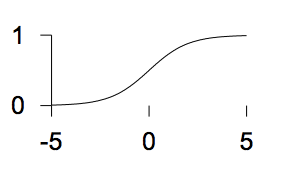 \(f(a) = \frac{1}{1+e^{-a}}\)
The sigmoid (tanh) function
 \(f(a) = tanh(a)\)
The step function
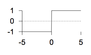 \(f(a) = \left\{
\begin{matrix}
1& a > 0\\
0& a \leq 0
\end{matrix}
\right.\)
\(f(a) = \left\{
\begin{matrix}
1& a > 0\\
0& a \leq 0
\end{matrix}
\right.\)
RELU
The RELU function
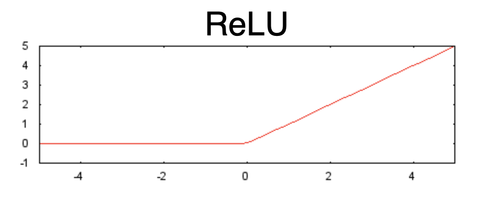
\(f(a) = \left\{
\begin{matrix}
a& a > 0\\
0& a \leq 0
\end{matrix}
\right.\)
Activity
The activity \(y=f(a)\) is the result of applying the activation function \(f()\) to the activation \(a\) (the weighted sum of inputs and weights).
Input layer
First introduced in b1_lecture.
The input layer is the one that receives the input data. For each data example, the input layer takes vector with a finite number of features described numerically with an embedding. The Input layer simply passes those features directly to the first hidden layer (or to the output layer if there are no hidden layers).
Output layer
First introduced in b1_lecture.
The output layers includes the predictions in the form of logits or softmax probabilities for all classes in the outcome.
Hidden layer
First introduced in b1_lecture.
A hidden layer appears anywhere between the input and the output layers. A hidden layer takes outputs of the previous layer as inputs and its outputs become the inputs to any subsequent layer.
Fully connected layer/dense layer
Embedding layer
Capacity
Resnet
Depth
The depth of a neural network is defined as the sum of the number of its layers, that includes the hidden layers and output layers, but not the input layers.
Pooling/sub-sampling
Model Training / Learning
Loss/Error function
First introduced in b0_lecture
A loss function quantifies the difference between an output predicted by the model \(h\) and the ground truth value \(y\) for each example \(x\)in a training set. Losses are used in supervised learning where training set data includes labels for the training examples providing the values the model tries to predict.
\[L(\theta, h(x), y)\]Empirical Risk
First introduced in b1_lecture.
The empirical risk is the average of the loss over a known training set \(\{x^n,y^n\}_{n=1}^N\). That is, the performance of the algorithm on a known set of training data.
\[R(\theta) = \frac{1}{N} \sum_{n=1}^N L(\theta, h^n(x), y^n)\]Cross-Entropy loss
First introduced in b0_lecture for a binary classification example.
For a given example, cross-entropy loss describes the predictions \(y^{(n)}=(y^{(n)}_1,\ldots y^{(n)}_I)\) and the labels \(t^{(n)}=(t^{(n)}_1,\ldots t^{(n)}_I)\) as two probability distribution, and it calculates the cross entropy between the two, averaged to all \(N\) examples as
\[L = - \frac{1}{N} \sum_{n=1}^N \sum_{i=1}^I t_i^{(n)} \log y^{(n)}_i.\]The cross entropy loss is always positive.
For standard classification using one-hot labels and softmax of logits (outputs), it becomes \(\mathbf{0}\) when the classification is perfect, that is, the true class achieves probability one. Larger values mean worse predictions. The cross-entropy loss can blow up and reach infinity if the models assigns near zero probability to the true class.
Binary Cross-Entropy loss (BCE)
In the particular case of only two possible outcomes (\(I=2\)), and the probability distributions for the outputs and labels are \(y^{(n)}=(y^{(n)},1-y^{(n)})\) and the labels \(t^{(n)}=(t^{(n)},1-t^{(n)})\), (with \(0\leq y^{(n)}\leq 1\) and \(0\leq t^{(n)}\leq 1\)), then the cross-entropy loss
\[L = - \frac{1}{N} \sum_{n=1}^N \left( t^{(n)} \log y^{(n)} + (1-t^{(n)}) \log (1-y^{(n)})\right).\]PyTorch has the function BCELoss() to calculate a Binary Cross-Entropy loss from probability outputs.
If the outputs come in the form of unnormalized logits \(y^{(n)}=(y^{(n)}_1,y^{(n)}_2)\) , then the function BCEWithLogitsLoss() performs first a softmax of the outputs, before calculating the BCE.
Softmax
The softmax function is a generalization of the logistic function to many dimensions.
For one value \(x\), the logistic function reports a value between \([0,1]\) given by
\[f(x) = \frac{1}{1+e^{-x}} = \frac{e^{x}}{1+e^{x}}.\]For a tuple \(x=[x_1,\ldots x_K]\), the softmax computes a tuple \(\sigma(x) = [\sigma_1,\ldots \sigma_K]\), given by
\[\sigma(x)_k = \frac{e^{x_k}}{\sum_{i=1}^{K} e^{x_i}},\]such that by constructions, each value \(\sigma(x)_k\) is a value between \([0,1]\), and
\[\sum_{k=1}^K \sigma(x)_k =1.\]That is the softmax of any tuple \([x_1,\ldots x_K]\) defines a probability distribution over all the possible values.
Entropy
For a given discrete probability distribution, the entropy is given by
\[H(p) = - \sum_n p_n \log p_n.\]The entropy of a probability distribution is always positive. Entropy measures the average information content of the probability distribution.
For uniform distribution \(p=(1/N,\ldots,1/N)\) is the probability distribution with the largest entropy given by
\[H(\mbox{uniform}) = -\sum_n \frac{1}{N} \log{\frac{1}{N}} = \log N.\]Perplexity
For a given discrete probability distribution, the perplexity is given by the exponent of this entropy
\[P(p) = exp H(p) = e^{-\sum_n p_n \log p_n} = e^{\sum_n \log (p_n)^{-p_n}} = \prod_n (p_n)^{-p_n}.\]epoch
An epoch is one complete pass of the learning algorithm over the entire training set. An epoch consits of a number of minibatch optimization steps. Each minibatch consists of a small random sample (sampled without replacement) from the training set.
masking
Gradient Descent
The gradient descent algorithm takes the gradient of an loss (error) function \(L\) with respect to the weights of a layer \(w\), \(g = \frac{\delta L}{\delta w}\) and descends the parameters against that gradient
\[w = w - \eta\, g\]\(\eta\) is called the learning rate
Batch GD
First introduced in b0_lecture
Here the gradient is calculated summing the contributions of all the examples in the training set.
Stochastic Gradient Descent (SDG)
The gradient is calculate considering a random subset (a batch) of the examples in the training set.
on-line GD
First introduced in b0_lecture
Here parameter updates is calculated after calculating the gradients with respect to one random example in the training set.
on-line GD is a type of SDG.
Backpropagation
First introduced in b0_lecture
The backpropagation algorithm calculates the derivatives of a loss (or error) function \({L}\) with respect to the weights at a given layer \(w_i\).
\[\frac{d L}{d W_i} := d W^i.\]Calculating these derivatives can be complicated. The loss depends explicitly only on the outputs of the last layer, \(y^N\), which depend explicitly on the layer activation which depend explicitly on the weights of the last layer. So calculating the derivative of the Loss respect to the weight of the last layer is
\[L \rightarrow y^N \rightarrow a^N \rightarrow W^N\]then,
\[d W^N := \frac{d L}{d W^N} = \frac{\delta L}{\delta y^N} \frac{\delta y^N}{\delta a^{N}}\frac{\delta a^N}{\delta W^N}\]Going down to layer \(N-1\) we have the explicit dependencies
\[L \rightarrow y^N \rightarrow a^N \rightarrow y^{N-1} \rightarrow a^{N-1} \rightarrow W^{N-1}\]then,
\[d W^{N-1} := \frac{d L}{d W^{N-1}} = \frac{\delta L}{\delta y^N} \frac{\delta y^N}{\delta a^{N}}\frac{\delta a^N}{\delta y^{N-1}} \frac{\delta y^{N-1}}{\delta a^{N-1}}\frac{\delta a^{N-1}}{\delta W^{N-1}}\]which generalizes for any inner layer weights \(W^i\) as
\[d W^{i} := \frac{d L}{d W^{i}} = \frac{\delta L}{\delta y^N} \frac{\delta y^N}{\delta a^{N}}\frac{\delta a^N}{\delta y^{N-1}} \frac{\delta y^{N-1}}{\delta a^{N-1}}\frac{\delta a^{N-1}}{\delta y^{N-2}} \ldots \frac{\delta y^{i}}{\delta a^{i}}\frac{\delta a^{i}}{\delta W^{i}}\]The chain rule
The chain rule is a method is calculus to calculate the derivative of a function \(f\) that depends on a variable \(x\) through another function \(g(x)\) as \(f(g(x))\).
Then the derivative of \(f(g(x))\) with respect to \(x\) is given by
\[\frac{d f}{d x} = \frac{d f}{d g} \frac{d g}{d x}.\]The chain rule also applies to partial derivatives, as it is the case of backpropagation
\[\frac{\partial f}{\partial x} = \frac{\partial f}{\partial g} \frac{\partial g}{\partial x}.\]Vanishing gradient
Layer Normalization
Batch Normalization Layer
Masking
Adam optimization
Forward pass
First introduced in b1_lecture.
The forward pass refers to the inference process. Given an input \(x\) , and a neural network with a set value of all parameters \(W\), the forward pass calculates \(y(x,W)\).
Backward pass
First introduced in b1_lecture.
The backward pass refers to the optimization of the weights using gradient descent or other algorithm. One needs the forward pass first in order to do the backward pass. One also need to define a loss to do a backward pass.
The backward pass starts from the last layer by calculating the change of the Loss with respect to the last layer weights. Those are needed to move the the previous layer and do the same gradient calculation. The backward pass continues until it reaches the first layer of the model.
Pre-training vs Fine-tuning
Foundational model
Regularization
First introduced in b0_lecture
Regularization is a collection of techniques used in the process of training a neural network in order to avoid overfitting to perform so well in the training data, to the detriment of its performance on other examples not seen at training (generalization)
There are different regularization techniques. The overall idea is to modify the objective function (the error or loss) so that it incorporates a bias against the solutions that favor the training set.
Early stopping
Dropout
A regularization technique that ignores (sets to zero or “drops”) a random fraction \(p\) of the input features during training.
nn.dropout(p=0.3)
means that 30\% of the features will be dropped. A Dropout layer is used only during training. Dropout layers are usually placed after fully connected or CNN laters.
L_1 regularization
L_2 regularization
Ablation
overfitting
In machine learning overfitting referees to the fact that for models with many parameters is is possible to fit the parameters too well to the training data in a way that the performance of the model in data that has not been seen at training is very poor.
Overlap between the training and the testing sets is often referred to as data leakage.
Proper testing of models performance requires to train and test the model on sets of sequences that are not similar to each other. Deciding what that similarity implies can be complicated.
data leakage
Refers to the situation in which the training set used to train a model, and the test set used to benchmark the method share examples, or examples are very similar between the two sets. Data leakage can be responsible for methods to appear to perform better than they would do if the test examples did not share any similarity with the training ones.
Generalization
Interpretability
Learning
First introduced in b0_lecture
Learning is equivalent to adjusting the parameters (weights) of the network such that the outputs \(y(n)\) of the network are optimized for all \(n\) training examples.
Learning requires the existence of a learning rule that specifies the way in which the neural network updates the weights in training.
Learning rule
The learning rule specifies the objective by which the parameters of the network will be updated in the training process. The learning rule depend on the inputs and the model parameters. In supervised learning, it also depends on the labels provided with the training data.
For instance, in our b0_lecture apples and oranges example, the learning rule is the cross entropy loss.
Learning rate
First introduced in b0_lecture
The learning rate refers to the proportionality value \(\eta\) that measures how fast weights are changed against the gradient of the loss \(g = \frac{\delta L}{\delta w}\).
\[w = w - \eta\, g\]If the learning rate \(\eta\) is very small, it may take too long to find the optimal parameters. If the learning rate is too big, then the system may bounce back an forth never reaching the optimal region for the parameters.
The learning rate is an example of the hyperparameter
Supervised Learning
First introduced in b0_lecture
In supervised learning, the objective is to adjusting the parameters (weights) of the network such that the output \(y(n)\) of the network is close to the label \(t(n)\) for all \(n\) examples.
Unsupervised Learning
Semi-supervised Learning
Adaptive Learning
Adversarial Learning
Zero-shot learning
Denoising
Distillation
Cross validation
Model Architecture
Autoregressive model
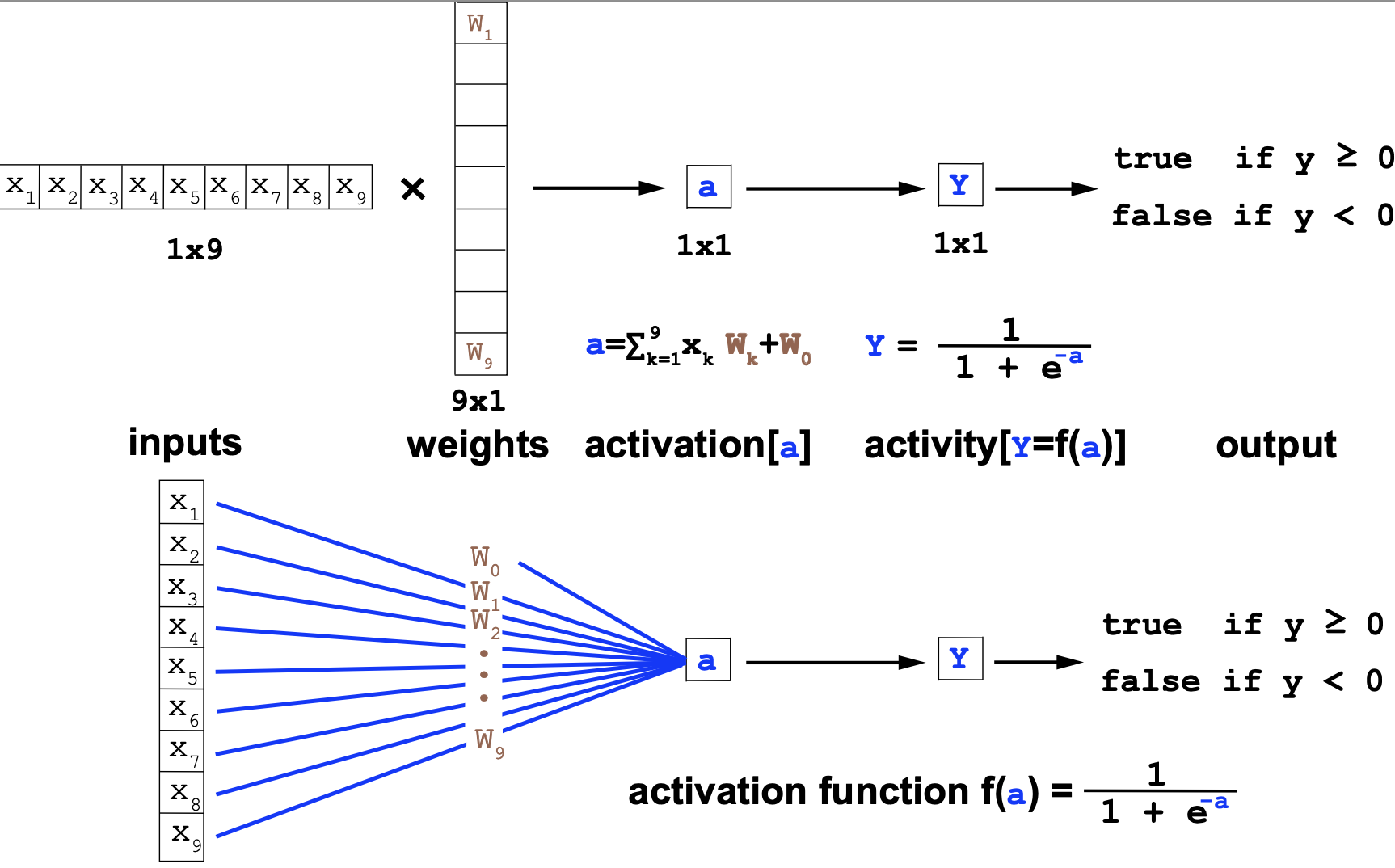
Perceptron
The perceptron is the simplest neural network consisting only of one neuron. We introduced the perceptron in the b0_lecture
Here are two equivalent representations of a perceptron with 9 inputs \(\{x_i\}_{i=1}^9\), 9 weights plus \(\{W_i\}_{i=1}^9\), one bias \(W_0\), and using sigmoidal activation.
MLP
Multilayer perceptron, introduced in b1_lecture
CNN
Convolutional neural networks, introduced in b2_lecture.
Residual Network
Residual networks, introduced in b2_lecture.
RNN
Recurrent neural networks, introduced in b2_lecture.
Attention
Transformer
Language model
Encoder
Decoder
Autoencoder
VAE
GAN
Generative model vs Discriminative model
Others
Homology
In sequence analysis, homology refers to sequences that share a common ancestor. We usually measure homology by programs that estimate sequence similarity above random expectations.
To train models in molecular biology specially RNA and protein sequences, it is important to also consider structural homology. Two proteins or two RNAs may not have much sequence similarity and still fold into very similar structures and be real homologs.