MCB128: AI in Molecular Biology (Spring 2026)
(Under construction)
(Now hiring TFs Fall 2026)
- Convolutional Networks (CNNs)
- Residual Networks (RNs)
- Recurrent Neural Networks (RNNs)
block 2:
Convolutional Networks, Residual Networks & Recurrent Networks / DNA/RNA binding motifs
In this block we introduce convolutional neural networks CNNs, recurrent networks RNs and recurrent neural networks (RNNs).
Convolutional Networks (CNNs)
For this section, we follow chapter 10 in Understanding Deep Learning. The molecular biology question associated to CNNs is that of RNA and DNA biding sites in proteins. We will follow the implementation of the method DeepBind “Predicting the sequence specificities of DNA- and RNA-binding proteins by deep learning”. We will also study how CNNs learn the sequence motifs motifs with this work: “Representation learning of genomic sequence motifs with convolutional neural networks”.
Multilayer perceptrons process all the input data together as a whole. Convolutional networks allow to process different parts of the input independently from each other using parameters shared by the whole input. CNNs have been extensively used to extract information from 2D images, such as where is the horse in the image? In molecular biology, CNNs have been used to recognize small motifs sequences found in genomes, such as transcription factor binding sites.
Convolutional Networks in 1-D
Convolutional networks are based on convolutional operations.
The convolution operation

Figure 1. 1D convolution with kernel of size 3.
For a vector \(x[D]\) and a set of weights of dimension K=3, \(w[3] = (w_1,w_2,w_3)\), usually referred to as the kernel, a convolution \(z\) (Figure 1) is defined as a weighted sum of the nearest three inputs,
\[\begin{aligned} z_i &= x_{i-1} * w_1 + x_{i} * w_2 +x_{i+1} * w_3\\ &= \sum_{j=1}^3 x_{i+j-2} w_j. \end{aligned}\]Each element in the output vector \(z[D]\), is a linear combination of the nearest three inputs with the same set of weights
\[z_2 = x_{1} * w_1 + x_{2} * w_2 +x_{3} * w_3,\\ z_3 = x_{2} * w_1 + x_{3} * w_2 +x_{4} * w_3,\\ z_4 = x_{3} * w_1 + x_{4} * w_2 +x_{5} * w_3.\\\]Padding
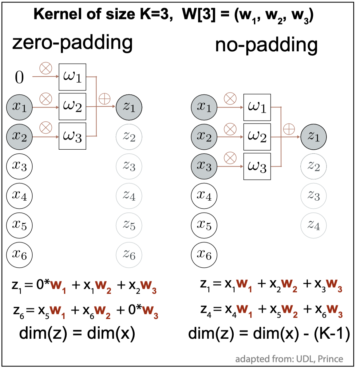
Figure 2. Edge cases in 1D convolution with kernel of size 3. Solutions: zero-padding (left), the dimensions of the inputs and outputs remain the same. No padding (right), the dimension of the output is smaller than the input by K-1 = 2.
For the edge cases, the convolution kernel extends beyond the inputs. Two typical solutions to deal with edge cases are given in Figure 2.
-
zero-padding. It extends the inputs by \(\frac{K-1}{2}\) additional entries above the first input value and also below the last input value. These extra input entries are valued to zero.
-
no padding. Only non-zero convolutions are considered. In this case, the dimension of the resulting outputs is smaller than that of the inputs.
Kernel size, stride, dilation
-
The weights that define a convolution constitute the kernel of the convolution. In 1D, the kernel is a vector of dimension \(K\), \(W[K]=(w_1,\ldots.w_K)\). In 2D a convolutional kernel is defined by a matrix \(W[K,K]\). The kernel dimension is usually an odd number so that it can be centered around the middle position.
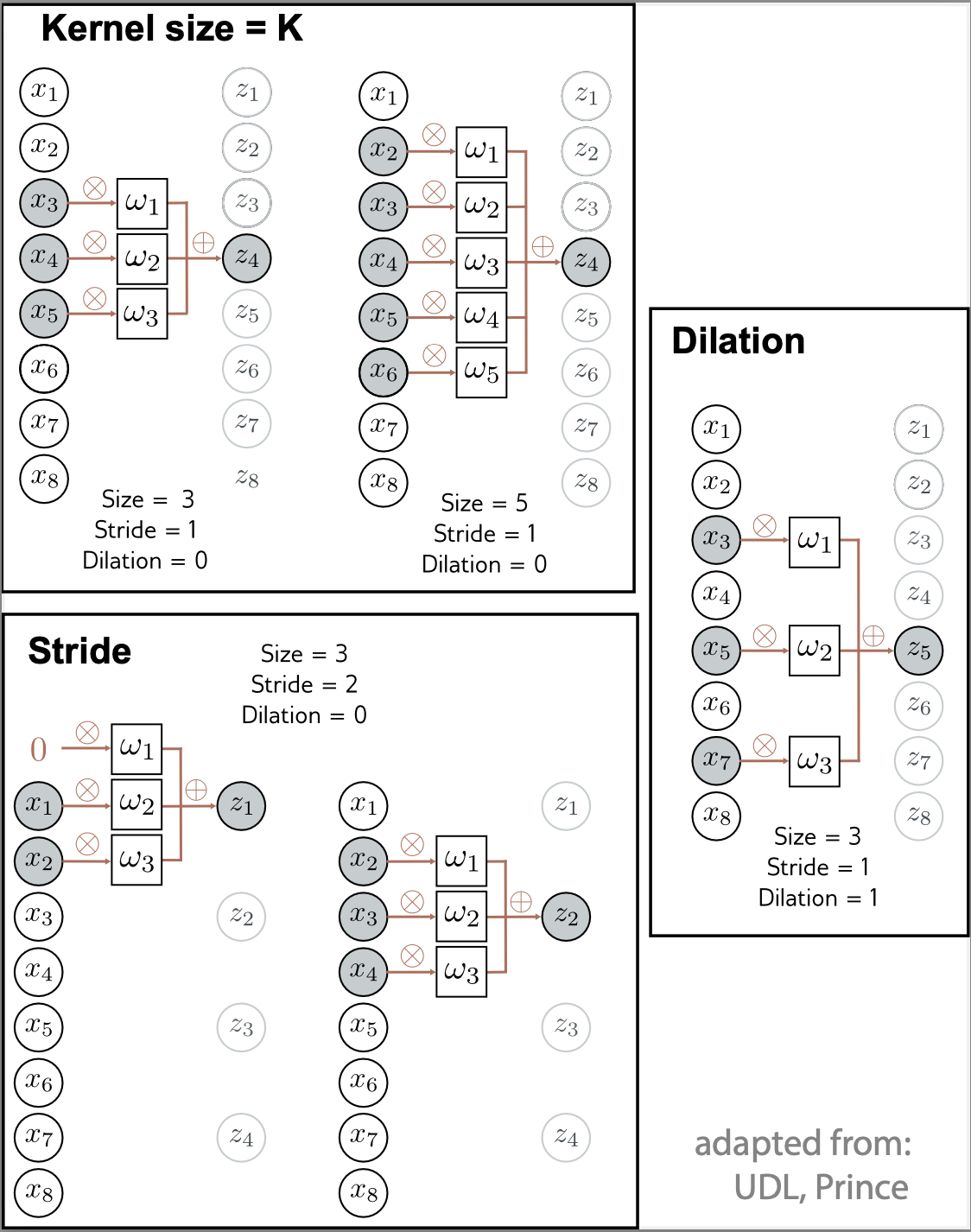
Figure 3. -
As the kernel is applied to the inputs, the stride define how many positions we skip when we go from one convolution to the next. A stride of one, result on a output of the same dimension than the input (using zero-padding). A stride of two, will result on an output with about half the number of outputs
-
A dilation results when a convolution is not applied to contiguous inputs but some inputs are left out. The number of inputs ignored between the weights determines the dilation rate. When the weights are applied to consecutive inputs, that determines a dilation rate \(=0\).
Equivariant by translation
A convolution is equivariant to a translation, which means that the input changes the same way as the output when subject to a translation.
Figure 3B. A convolution is equivariant to translations. A convolution with position dependent biases is not.
where \(T_m(x_n)\) represents a translation from input \(x_n\) to input \(x_{n+m}\).
This property is important. Consider the case of detecting a subsequence motif in a genome. Translational equivariance implies that if the motif is shifted to a differnt position in a different genome or if it appears in different locations within the same genome, the CNN will detect the motif in its new location with the same score.
Figure 3B shows that, because the weights in a CNN are independent of the location at which they are applied to the input, the network is translationally equivariant. Figure 3B also show an example of how translational equivariance is broken if the kernel weights have a dependence on the location where they are applied.
Convolutional layer
A convolutional layer, takes inputs \(x[L]\), and calculates its outputs \(y[L]\) by convolving the inputs with a convolutional kernel \(W\) of size \(K=\) adding a bias \(\beta\), and passing it through an activation function \(f\),
\[y_l = f\left( \beta + \sum_{k=1}^K x_{l+k-(K-1)} w_k\right),\]which for the particular case \(K = 3\), results in (Figure 1)
\[y_l = f\left( \beta + x_{l-1} w_1 + x_{l} w_2 + x_{l+1} w_3\right).\]Pooling
Most convolutional networks include one additional layer after the convolutional layer (with activation) another layer in order to downsample the inputs. Subsampling is convenient because it increases the receptive field of the convolution.
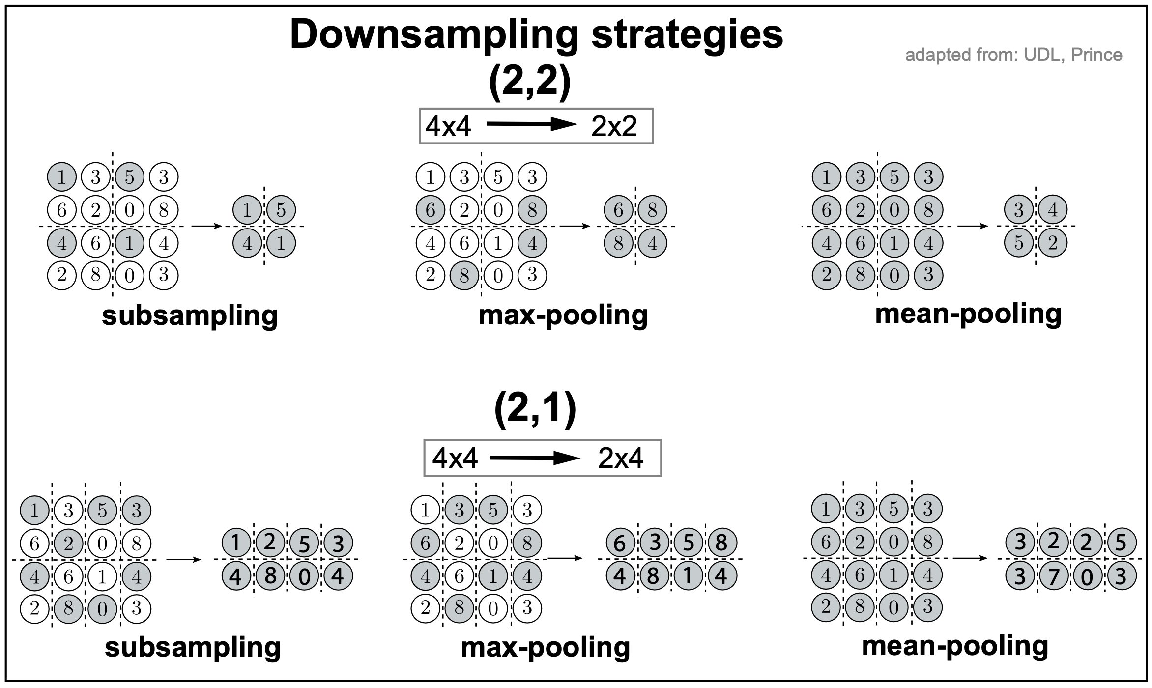
Figure 4.
There are several forms of downsampling, described in Figure 4 with two examples for a 4x4 input, one downsizing (2,2) to at 2x2 input, the other downsizing (2,1) to a 2x4 input.
-
random subsampling. Involves simply selecting randomly one of the input in each 2x2 or 2x1 block.
-
max pooling. In max pooling, we take the max of every 2x2 or 2x1 block.
-
mean pooling. In mean pooling, we take the average of every 2x2 or 2x1 block.
Channels
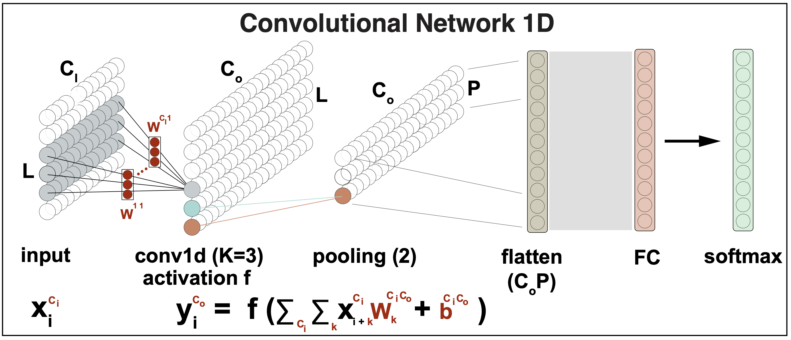
Figure 5.
Typically, multiple convolutions are applied to the input \(x\) and stored in channels.
When two convolutions \(W^1[3]\), \(W^2[3]\) are applied to the same input, that results in two channel outputs
\[y^1_i = f\left(\beta^1 + \sum_{k=1}^3 x_{i+k-2} W^1_k\right)\\ y^2_i = f\left(\beta^2 + \sum_{k=1}^3 x_{i+k-2} W^2_k\right)\\\]which generalizes to \(C_o\) channel outputs as
\[y^{c_o}_i = f\left(\beta^{c_o} + \sum_{k=1}^3 x_{i+k-2} W^{c_o}_k\right)\quad for\, 1\leq c_o \leq C_o\]Moreover, the inputs can also have many layers \(C_I\), then the hidden units in each output channel are computed as a weighted sum over all \(C_i\) channels and K kernel entries using a weight matrix \(W[K,C_I]\).
\[y^{c_o}_i = f\left( \sum_{c_i=1}^{C_I} \left[\beta^{c_i c_o} + \sum_{k=1}^3 x_{i+k-2} W^{c_i,c_o}_k\right]\right)\quad for\, 1\leq c_o \leq C_o\]In general, the input and hidden layers all will have multiple channels (Figure 5). If there are \(C_I\) input channels and \(C_O\) output channels, then we need \(W[K,C_I,C_O]\) weights, and \(\beta[C_I C_O]\) biases.
For instance, in the case of biological sequences like DNA or RNA, it is typical for the input to have four channels (\(C_I=4\)), one for each of the nucleotides.
The end of a CNN
As described in Figure 5, the final layers of a CNN usually involve flattening the output of the last CNN layer, and then applying a fully connected layer to obtain the desired output dimension, in which to perform a softmax output to be used for output classification.
For instance, in a model to predict sequence motifs, as it is the case for the DeepBind model we describe later, the output dimension is the number of motifs that the model is expected to detect.
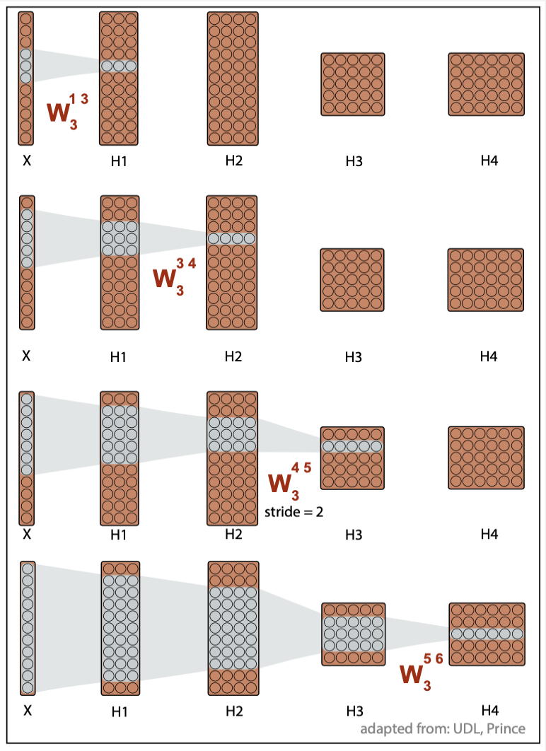
Figure 6.
The receptive field
The receptive field of a given layer is defined as t the extent of inputs that feed into any element of that layer.
For instance, consider Figure 3 that includes 4 hidden layers, and uses CNN kernels of size \(K=3\).
-
Each element of the first layer \(H_1\) includes a weighted sum of three inputs, thus the receptive field of \(H_1\) is 3.
-
Each element of the second layer \(H_2\) includes a weighted sum of three elements for each channel of \(H_1\), which are themselves weighted sums of three inputs, and the receptive field of \(H_2\) is 5.
-
The receptive field of \(H_3\) is 7.
-
The receptive field of \(H_4\) is 11, the whole input.
The receptive field of successive layers is constantly increasing, thus allowing for the integration of more and more data. For that reason, most CNN models often include several convolutional layers before the elements of the last layer are feed to a fully connected layer and the outputs are reported as softmax probability values for classification.
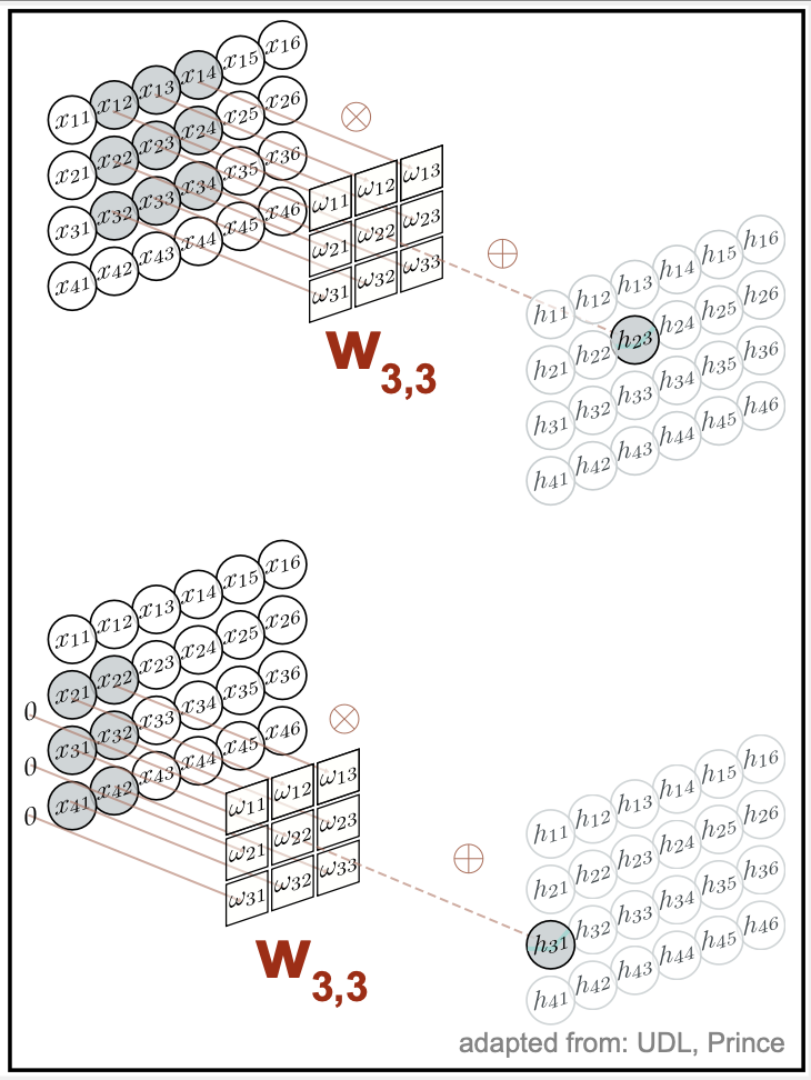
Figure 7. A 2D convolutional layer. Each output computes a weighted sum of the 3×3 nearest inputs, adds a bias, and applies an activation function.
CNN for 2D inputs
All the results presented this far describe convolutional networks applied to input data in 1D. Most results generalize for data in 2D (such as images), and even to 3D (applied to volumes such as medical imaging), or even higher dimensions.
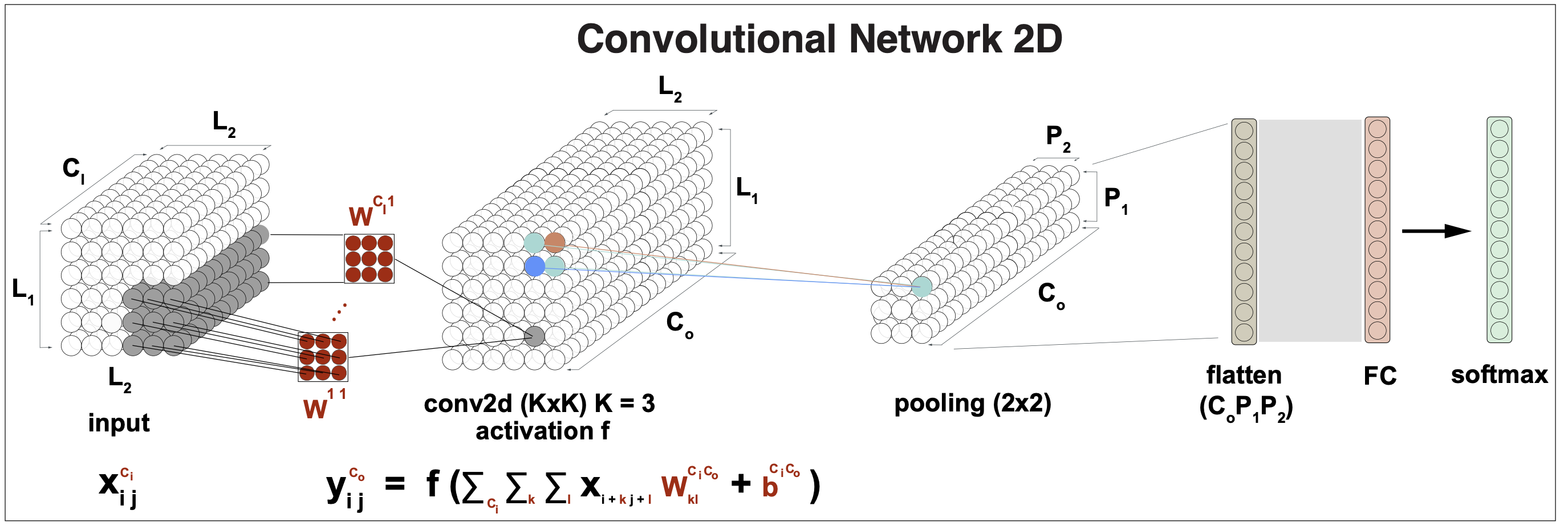
Figure 8. A CNN layer for 2D input data. Kernel size is 3.
For 2D inputs \(\{x_{ij}\}\) for \(1\leq i \leq L_1\) and \(1\leq j\leq L_2\), and a \(K\times K\) convolution kernel \(W\), the \(L_1\times L_2\) outputs \(y_{ij}\) (assuming zero-padding), are given by (assuming \(K=3\)),
\[y_{i,j} = f\left( \beta + \sum_{k=1}^3 \sum_{l=1}^3\, x_{i+k-2 j+l-2} W_{kl}\right).\]A convolution for 3D inputs requires kernels \(W[K, K, K]\), and this results generalizes to higher dimensions.
The 1D result for \(C_I\) input channels producing \(C_O\) output channels also generalizes. A CNN for 2D data, require \(K\times K\) kernels for each input and output channel, \(W[C_I C_O, K, K]\),, as described in Figure 8.
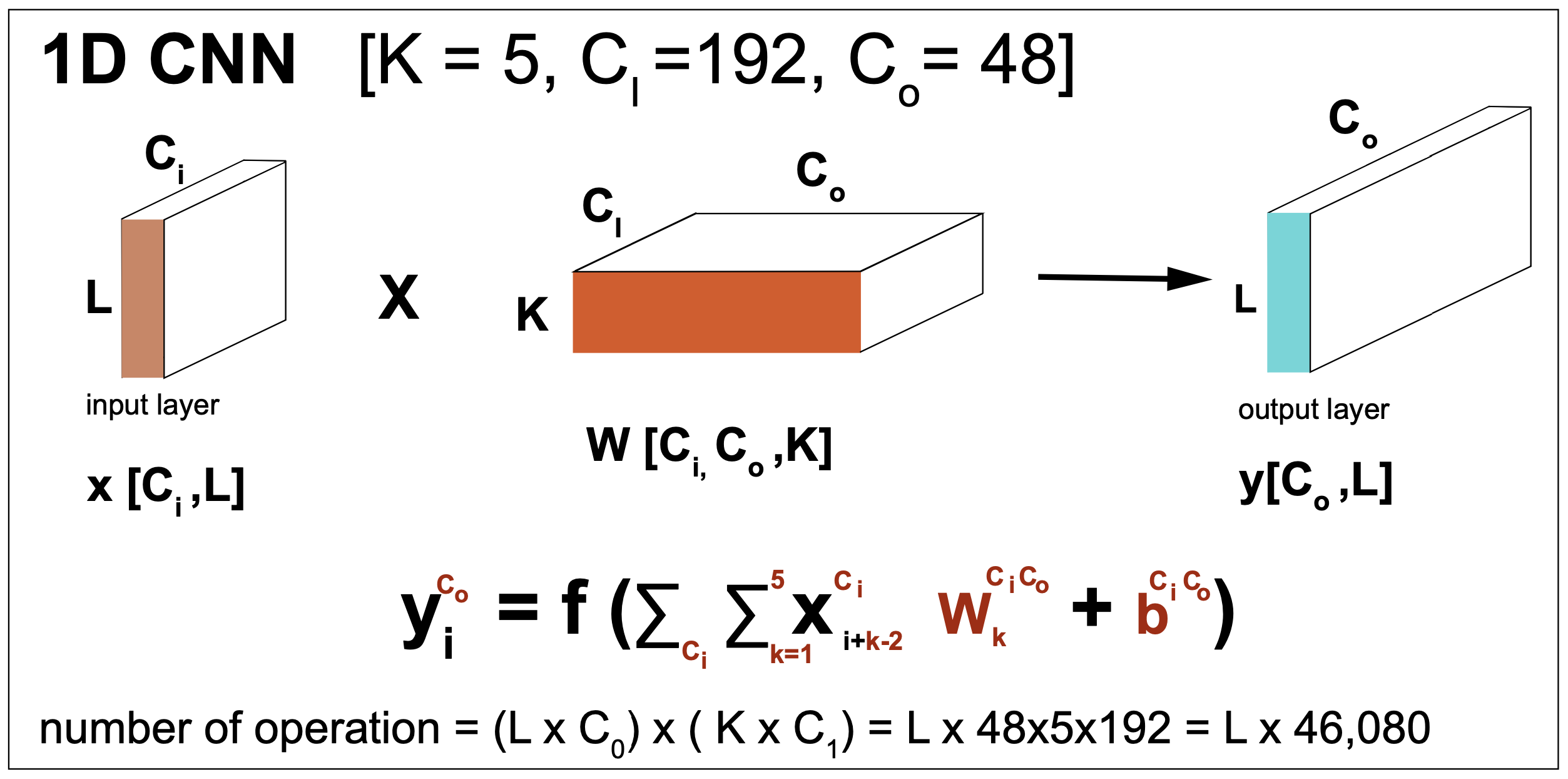
Figure 9. A CNN layer for 1D input data in numbers. A generic activation function is represented by f. The result generalizes for more input dimensions by replacing L and K in the vectors where they appear. We assume zero-padding so that the input and output dimensions remain identical.
A CNN layer in a nutshell
Figure 9 gives a description of the tensors and operations involved in a CNN layer. The input can have an arbitrary number of channels \(C_I\), and the output can also have arbitrary dimension \(C_O\). This CNN layer requires \(K\times C_I\times C_O\) weights \(w\) and \(C_I\times C_O\) biases \(\beta\).
DeepBind, DNA/RNA binding motifs
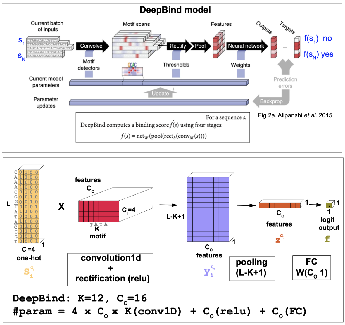
Figure 10. The DeepBind model.
This is the code that implements the basics of the DeepBind model.
The DeepBind model is a CNN method introduced by Alipanahi et al. in 2015 to predict DNA and RNA binding sites of specific proteins such as transcription factors. The method is best described in this supplemental file. See Figure 10 for more details.
The inputs
The inputs are DNA or RNA sequences \(s\) (of lengths ranging from 14-101 nts in their experiments) that are 1-hot encoded, that is there are \(C_I=4\) input channels.
\[S_i^{C_i} \quad 1\leq i\leq L \quad C_i = \{1,2,3,4\}\]The outputs
For each input sequence \(s\), the output is just one single value \(f(s)\).
If the model has been trained on positive and negative examples of sequences including one particular motif, then \(f(s)\) is transformed to a probability using the linear logistic function
\[\sigma(f) = \frac{1}{1+e^{-f(s)}}\]The model architecture
- A 1D CNN. The input has dimension the length of the sequence, and it uses 4 input channels, one for each nucleotide (a one-hot) encoding. The number of output channels \(C_O\) is set to 16, and it is referred to as the number of features. The kernels have size \(K=12\), and thus the total number of CNN parameters is \(W[C_I,C_O,K] = W[4,16,12]\).
The 1d convolution without padding results in
\[x_i^{C_o} = \sum_{C_i=1}^{4} \sum_{k=1}^K W_{k}^{C_i C_o} S_{i+k} ^{C_i} \quad 1\leq i\leq L - K +1\]- A RELU activation function with a set of weights \(b^{C_O}\) (that need to be trained). DeepBind uses a RELU activation function
- Pooling DeepBind pools all \(L-K+1\) features into one value by max-pooling
DeepBind applies a very large pooling size which results in the largest possible receptive field. This is ok because DeepBind only attempts to predict if the input sequence contains some binding site. However, this does not give any resolution to determine where within the sequence is the motif placed. In order to have that level of precision, one needs to use smaller pooling sizes. In the homework we analyze the trade-offs between large receptive fields and motif determination.
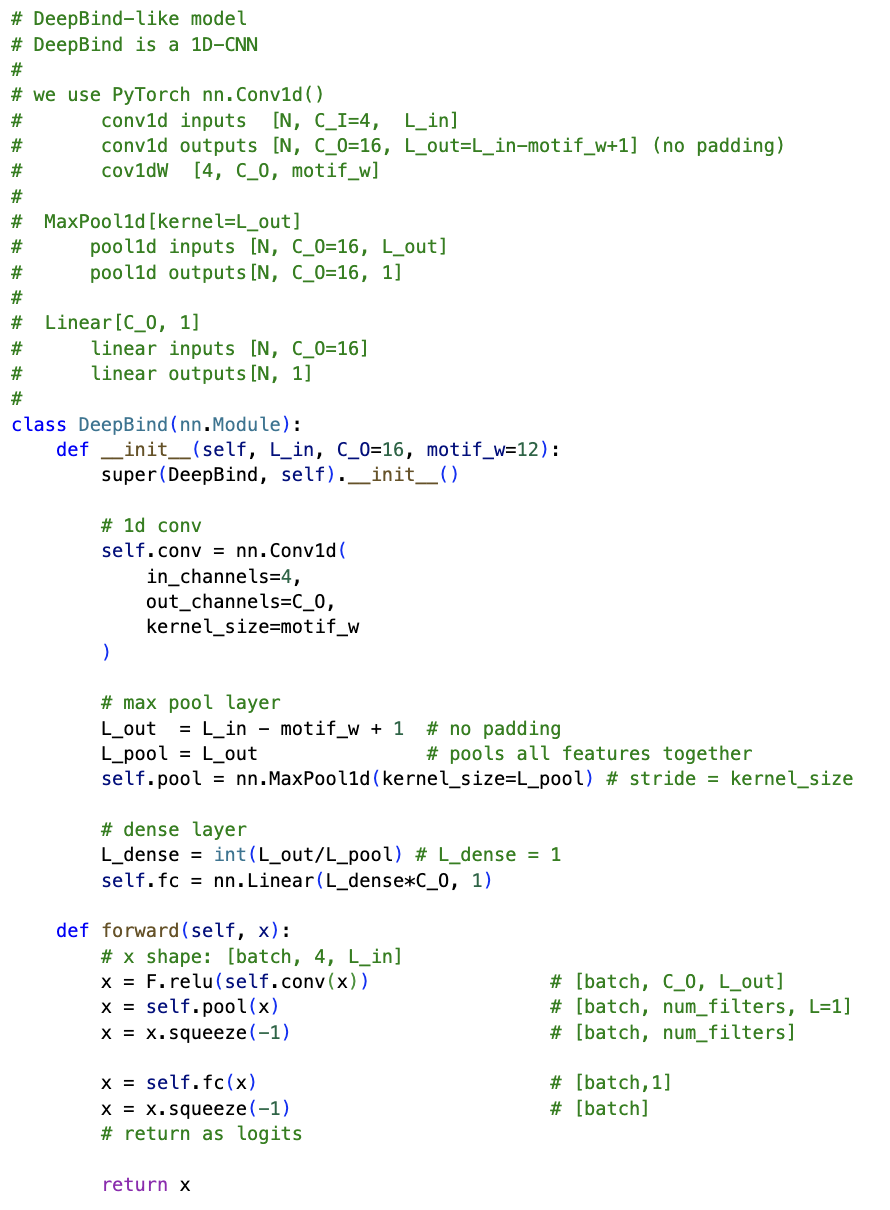
Figure 11. PyTorch code for the fundamentals of the DeepBind method to identify motifs in biological sequences.
- A FC layer Finally a Fully connected layer with weights \(W^{C_O}\) is applied to produce one single logit output
The training
Training was done using mini-batch stochastic gradient descent, updating the parameters with Adam updates.
The loss function used for this two-class classification problem is standard binary cross-entropy
\[BCELoss(\sigma(f)) = BCEWithLogitsLoss(f) = - \left[t \log(\sigma(f)) + (1-t)\log(1-\sigma(f))\right]\]where \(\sigma(f)\) is the logistic function
\[\sigma(f) = \frac{1}{1+e^{-f(s)}}.\]The code
Here is the code that implements the basics of the DeepBind model. Figure 11 shows a snippet of our simplified DeepBind code.
DeepSEA, DNA/RNA binding motifs
The method DeepSEA introduced in “Predicting effects of noncoding variants with deep learning based sequence model” is another method to learn regulatory sequences with very similar design to DeepBind by using a combination of convolutional layers, followed by pooling and fully connected layers.
Residual Networks (RNs)
For this section, we follow chapter 11 in Understanding Deep Learning.

Figure 12. A sequential network.
The models we have introduced so far are all sequential, the output of a convolutional block feeds into a FC linear network which feeds into a second CNN block, and that can go on for many iterations. The problem of these sequential networks (Figure 12) is that the gradients of the output (needed to do backpropagation and update the parameters in training) wrt to early layers become increasingly complex. As we have to multiply more and more small terms, eventually the gradients become negligible and the training stop working. This is referred to as the vanishing gradient problem.
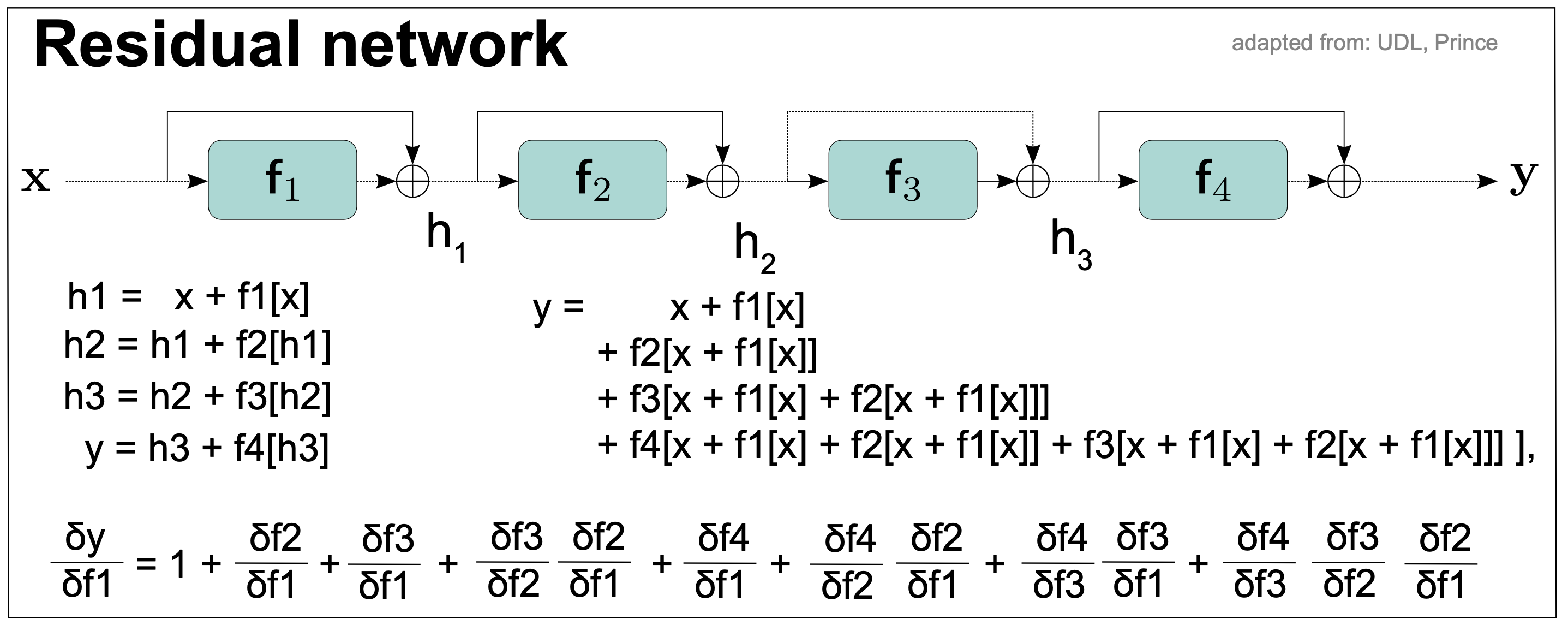
Figure 13. A residual network.
Residual connections
Residual networks alleviate the exploding/vanishing gradient problem. As we see in Figure 13, each layer adds to the previous value (creating a residual) rather than completely transforming the value.
The residual network is defined by the connections
\[\begin{aligned} h1 &= x + f1(x)\\ h2 &= h1 + f2(h1)\\ h3 &= h2 + f3(h2)\\ y &= h3 + f4(h3)\\ \end{aligned}\]Each additive combination of the input and the processed output is known as a residual block or residual layer.
By making all substitutions in the above equations, we obtain
\[y = x + f1(x) + f2 \left(x + f1(x)\right) + f3 \left( x + f1(x) + f2 (x + f1(x))\right) + f4 \left( x + f1(x) + f2 (x + f1(x)) + f3 (x + f1(x) + f2(x + f1(x))) \right)\]thus, the output \(y\) depends directly on the first layer \(f1\), in addition to other indirect contributions through other layers. That means that changes in the first layer \(f1\) contribute directly to changes in the output which helps alleviate the vanishing gradient problem.
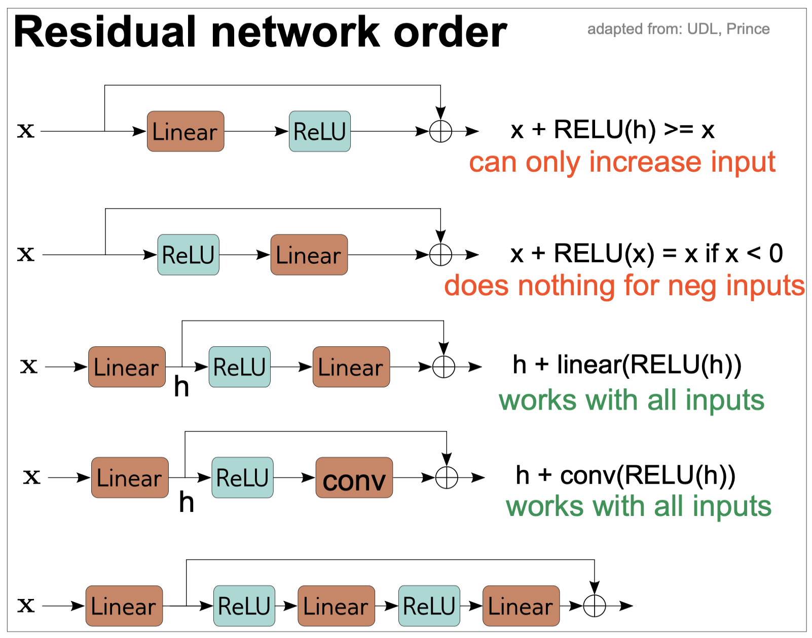
Figure 14. Order of operations in residual networks.
Residual Network order
In any neural network, we need to introduce non linear activation functions such as RELU so that the entire network is not linear.
In a typical neural network, the RELU function is at the end so that the output is not negative. However, if we do the same in a residual network, then each residual block all it can do is to increase the input (Figure 14). For that reason, in residual networks, the order is reversed and the RELU block goes in front of the linear (or convolution) block.
Moreover, if we start these blocks with a ReLU activation, then they will do nothing if the inputs are negative. To avoid that, it is common to start wit a linear transformation before any residual block, as seen in Figure 14.
Recurrent Neural Networks (RNNs)
All the networks we have seen so far, they have no concept of memory. All inputs are processed independently from each other. However, most actions occur following some sequence, one after the other. Think of talking or the ribosome translating a messenger RNA. Recurrent neural networks (RNNs) take a sequential approach by iterating over input elements.
RNNs for time series (biological sequences in our case)
RNNs take a sequence of inputs (nucleotides or amino-acid sequences in genomics) one at a time. At each step, the network receives both the new input and a hidden representation computed from the previous time instance. The final output contains information about the whole input.

Figure 15. A simple recurrent neural network (RNN) with a hidden layer.
A simple RNN
Figure 15 describes one of the simplest RNNs with one hidden state. We have an input \(X_t\in R^I\) per time step, and it also includes a hidden layer output \(H_t\in R^H\).
The calculation of the hidden layer output \(H_t\) depends on input \(X_t\) and also the output at the previous step \(H_{t-1}\),
\[H_t = \sigma\left(X_t W_{xh} + H_{t-1} W_{hh} + b_h\right),\]where \(\sigma\) is the activation function.
The output of the output layer is given by
\[O_t = H_t W_{ho} + b_o\]Thus the parameters of a RNN with one hidden layer are
\[W_{xh}\in R^{I\times H}\\ W_{hh}\in R^{H\times H} \\ W_{ho}\in R^{H\times O}\\ b_h\in R^{H}\\ b_o\in R^{O}\]In our applications of RNNs for sequence data, the tokenization of a DNA, RNA or protein sequence into nucleotides/amino acids is obvious. Each element of the time series is one of the consecutive residues in the biological sequence.
One important problem of RNNs is that they can forget information that is far back in the sequence. To alleviate that problem other more sophisticated RNNs such as long short-term memory networks (LSTM) and gated recurrent units (GRUs) were introduced. Next we describe in detail long short-term memory networks RNNs.
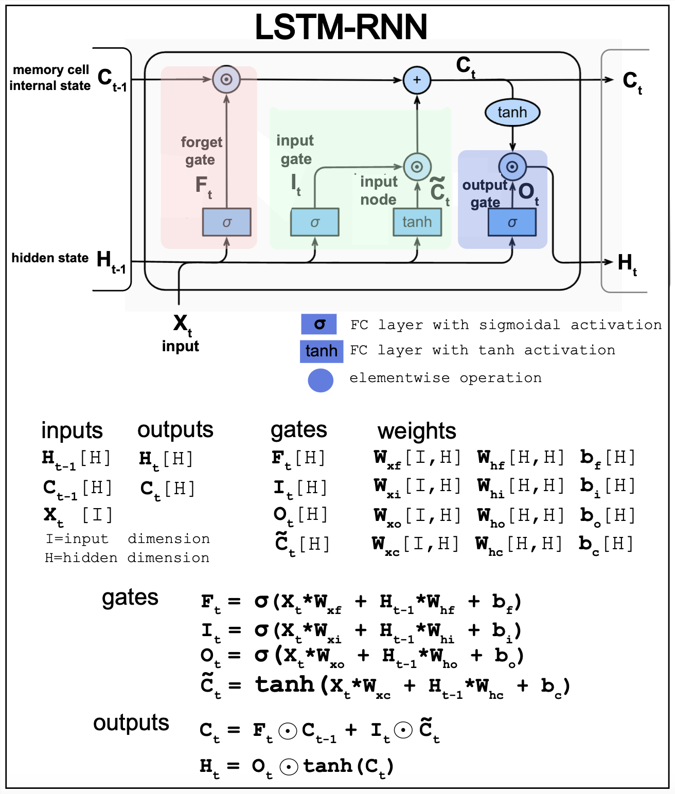
Figure 16. Long short-term memory (LSTM) RNN model.
LSTM-RNNs
The LSTM architecture is designed to remember information over long time periods. In a neural network, the activations are its short-term memory, and the weights are its long-term memory. LSTMs are designed to make short-term memory last longer. An LSTM replaces each unit in RNN with a memory block that determines when to store or forget information.
Figure 16 described the details of the LSTM architecture.
-
\(F_t\) controls how much of the previous memory \(C_{t-1}\) is retained.
-
\(I_t\) controls the new input \(X_{t}\) without any previous memory input.
-
\(\widetilde{C}_t\) creates a new memory which combined with the forget gate \(F_t\) generates the current memory \(C_t\).
-
\(O_t\) controls how much goes to the new hidden state \(H_t\)
PyTorch code that implements a simple RNN and a LSTM RNN can be found here. I have applied to the a similar dataset as the one used for DeepBind. The positives are DNA sequences with one particular motif embedded, and random sequences without any motif as negatives. In my hands and for the same data, the simple RNN has trouble identifying the sequences with the motif, but the LSTM-RNN is able to reach almost perfect classification
Code for RNNs
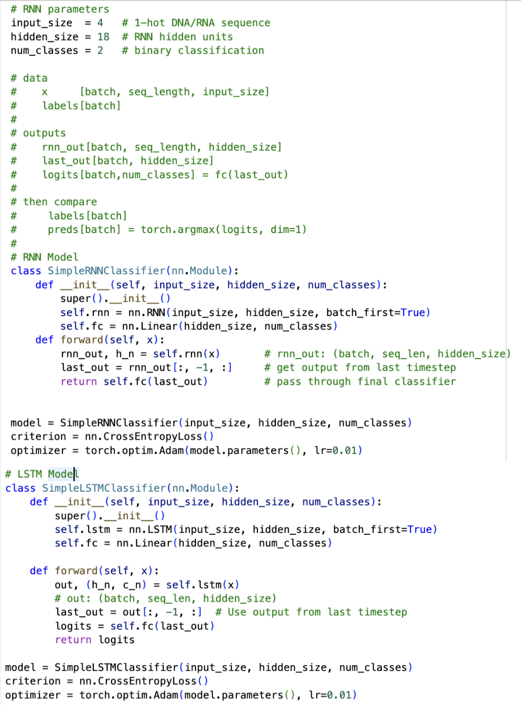
Figure 17. simpleRNN and LSTM-RNN basic PyTorch code.
Here is the code that implements a simple RNN and a LSTM-RNN. Figure 17 shows a snippet of that code.
DanQ functional motif identification using CNNs+bidirectional-LSTM-RNNs
As a biological example, we are going to consider the method DanQ which uses a combination of CNNs and LSTMs with the purpose of prediction non-coding functional elements in genomes. The idea is the the first CNN layers of the model will identify relevant motifs, and the later LSTM-RNN layers may learn information about how the motifs are arranged in the genome and their frequency of appearance.
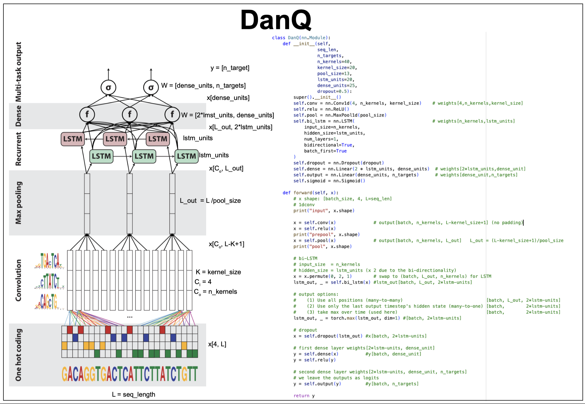
Figure 18. The DanQ model and code.
Input data
Each input is a \(1,000\) sequence from the human genome in one-hot format \(x[4,L=10000]\).
Training data
DanQ uses for training 919 sequence motifs (peaks) identified by using the methods ChIP-seq (Chromatin ImmunoPrecipitation followed by Sequencing) and DNase-seq (DNase I hypersensitive site sequencing) which are known to identify DNA sites associated to proteins such as transcription factors or histones.
Each training input is a 1,000 nt sequence centered around one of the 919 motifs. For each training input there is a one-hot target vector \(t\) of dimension \(n\_targets = 919\).
\[X[4,L=1000]\\ t[\mbox{n_targets}=919]\]Out training data
In our in class implementation, we have selected \(10\) known transcription factor (TF) DNA binding sites from the JASPAR database. Each motif has been embedded in a random sequence of length \(L=100\), and we have added one class for not having any motif. A similar number of samples have been taken for each of the \(11\) target classes.
So, each example of out training data has dimensions (which are customizable in the code)
\[X[4,L=100]\\ t[\mbox{n_targets}=11].\]The DanQ model
1d Convolutional layer (CNN) + relu
To detect relevant sequence motifs, it first uses a 1d convolution. The conv1d weight dimensions are \(W[4,\mbox{n_kernels},\mbox{kernel_size}]\), and using no padding, it produces, an output with \(L_{out} = L-\mbox{kernel_size}+1\), features,
\[X[4,L] \times W[4,\mbox{n_kernels},\mbox{kernel_size}] \rightarrow X[\mbox{n_kernels},L_{out}].\]For DanQ, \(\mbox{n_kernels} = 320\), and the \(\mbox{kernel_size} = 26\).
Max-pooling layer
The max-pooling layer by downsampling the feature dimension, is expected to help learn actual motifs.
\[X[\mbox{n_kernels},L_{out}] \rightarrow X[\mbox{n_kernels},L_{out}/\mbox{pool_size}].\]For the DanQ data, the pool size is set to 13, and the feature dimension after pooling becomes \(1000/13 = 75\).
bi-directional LSTM-RNN layer
The bi-directional LSTM layer has 320 units per direction. This layer is expected to capture how motifs are placed respect to each other.
\[X[\mbox{n_kernels}, L_{out}] \rightarrow X[L_{out}, 2*\mbox{lstm_units}]\]Dropout Layer
The DanQ method uses a dropout layer to help with regularization. It uses a dropout probability of 0.5.
Fully connected (FC) layer + relu
This layer integrates all information, and uses \(\mbox{dense_unit} = 925\),
\[X[2*\mbox{lstm_units}] \rightarrow X[\mbox{dense_unit}].\]Final FC layer + sigmoidal
This final layer output a vector of logits of dimension \(\mbox{n_targets} = 918\), which is the number of motifs to differentiate. The logits are converted through a sigmoid function to a probability distribution of possible outcomes for classification.