MCB128: AI in Molecular Biology (Spring 2026)
(Under construction)
(Now hiring TFs Fall 2026)
- Multilayer perceptron (MLP)
- Protein 2D structure
- Fundamentals of neural networks
- Generalization
- Appendix
block 1:
Feed Forward Networks / Protein 2D structure
In this block we introduce the Multilayer perceptron (MLP).
A good reference for the basics of deep learning is this book (pdf attached) Understanding DL. I strongly recommend it.
As a practical implementation of a MLP in molecular biology, we will study the work of Qian & Sejnowski (1988), “Predicting the secondary structure of globular proteins using neural network models” in which they use a MLP with one hidden layer to infer the secondary structure of globin proteins. This method is based on a previous work by the some of the same authors NetTALK applied to the problem of text-to-speech in which the inputs are strings of letters representing words and the outputs are sounds (phonemes). The MLP described by Qian & Sejnowski (1988) takes protein sequences as inputs, and reports as an output its secondary structure.
This is the code that implements the Qian-Sejnowski model.
Multilayer perceptron (MLP)
In the previous block 0, we discuss a one-neuron perceptron. We showed how perceptrons can work well as classifiers, when the inputs are linearly separable as in Figure9 of block 0. However, when the data is not linearly separable, it is provable that a simple perceptron cannot work. This result was introduced by Minsky & Papert in a book entitled “Perceptrons: An Introduction to Computational Geometry”, (1969).
Interestingly, that result halted research in neural networks for a while (the “ice age” of neural networks). The introduction of Multilayer perceptrons that can easily classify non-linearly separable, resolved the hiatus in the 1980s. I say interestingly, because Rosenblatt’s original perceptron paper from 1958 already includes “deep” neural networks with more than one layer of weights.
Generalization to many neurons, many layers and many outcomes
The single-neuron network can be easily generalized to be a fully connected neural network with many different outputs and going through many different layers from input to output.
The one-hot encoding of categorical variables
The states of our single-neuron network (active/inactive, apple/orange) can be easily rewritten using a one-hot representation.
\[\begin{aligned} \mbox{output/activity}\quad &\mbox{one-hot}\\ t = \{0,1\}\quad \quad &\bar t = [t_1, t_2]\\ t = 1\, \mbox{(Apple)} \quad &\bar t(A) = [1, 0]\\ t = 0\, \mbox{(Orange)}\quad &\bar t(O) = [0, 1]\\ \end{aligned}\]This one-hot representation easily generalizes for a categorical variable with more than two outcomes \(\{t_1,\ldots t_O\}\) as,
\[\bar t_1 = [1,0,\ldots,0]\\ \bar t_2 = [0,1,\ldots,0]\\ \dot\quad \\ \dot\quad \\ \dot\quad \\ \bar t_O = [0,0,\ldots,1]\\\]The output/activity: from a linear logistic function to softmax activation
The activation for the single-neuron,
\[a(\bar x,\bar W) = \sum_i x_i W_i + b,\]from which the output \(y\) ranging from zero to one is calculated using the liner logistic function
\[y = \frac{1}{1+e^{-a}}.\]The single activation \(a\) can be easily extended (for the same inputs) to more activations (“more neurons”) as
\[a_1(\bar x,\bar W^1) = \sum_i x_i W_i^1 + b^1\\ a_2(\bar x,\bar W^2) = \sum_i x_i W_i^2 + b^2\\\]and these activations can be easily converted into a \(2\)-dimensional probability outcome \(\bar y\),
\[\bar y = \{y_1,y_2\},\]such that \(y_1 + y_2 = 1\), and \(0\leq y_1, y_2 \leq 1\), using the softmax function
\[y_1 = \frac{e^{a_1}}{e^{a_1} + e^{a_2}}\\ y_2 = \frac{e^{a_2}}{e^{a_1} + e^{a_2}}.\]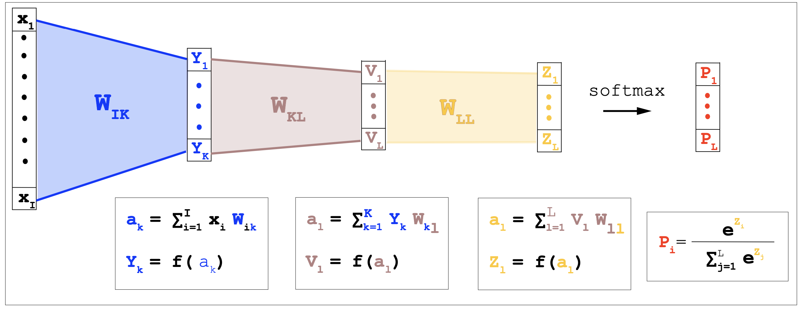
Figuren 1. A fully connected neural network with two hidden layers.
Neural network with many outputs
The above result generalizes easily to a network with many possible outcomes.
A \(O\)-dimensional activation \(\bar a\),
\[\bar a = \{a_1,\ldots, a_O\},\]can be converted to a probability vector \(\bar y\) using the softmax function
\[\bar y = \{y_1,\ldots, y_O\},\]such that
\[y_o = \frac{e^{a_o}}{e^{a_1} + \ldots + e^{a_O}}, \quad \mbox{and}\quad \sum_{o=1}^O y_o = 1.\]And the loss function \(G\) easily generalizes to the cross entropy between the true outcomes \((t^{(n)}_1,\ldots, t^{(n)}_O)\) and the predicted outcomes \((y^{(n)}_1,\ldots, y^{(n)}_O)\) summed to all \(1\leq n\leq N\) cases in the training set.
\[G(w) = - \frac{1}{N}\sum_{n=1}^N \sum_{o=1}^O t^{(n)}_o \log y^{(n)}_o(w).\]A fully connected (FC) layer
A fully connected (FC) layer connects every input in the previous layer to every output in the next layer.
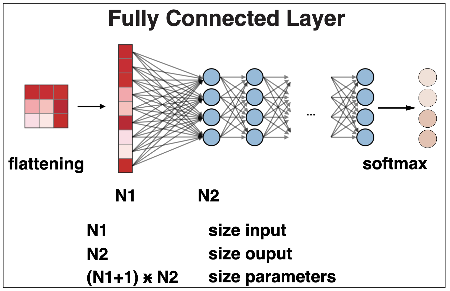
Figure 2. A fully connected layer. For an input layer of dimension N1, and an output layer of dimension N2, the weights of a FC layer have dimension N1*N2, plus a bias of dimension N2.
FC layers are typically used at the end of o a neural network to perform the final classification.
-
Flattening Before the data enters the FC layer, the possibly multi-dimensional input features are flattened into a single, one-dimensional vector.
-
Full connectivity Every neuron in the flattened vector is connected to every neuron in the FC layer, with each connection having its own weight.
-
Output The final FC layer typically uses a softmax activation function to output a probability for each possible classification label.
Some simple code describing these steps in a FC layer is provided here.
Protein 2D structure
In this section, we describe in detail the MLP with one hidden layer “Predicting the secondary structure of globular proteins using neural network models”, introduced by Qian & Sejnowski in 1988.
Protein secondary structure can be calculated based on its atoms’ 3D coordinates once the protein’s 3D structure is solved using X-ray crystallography or NMR. However, X-ray or NMR is expensive. Ideally, we would like to predict the secondary structure of a protein based on its primary sequence directly, which has had a long history.
The secondary structure of a given protein is described in Figure 3. It consists of mainly three possible local configurations that repeat over and over again: the alpha-helix, the beta-sheets and finally the random coil. The protein 2D structure is an intermediate between the protein sequence and the actual 3D structure.
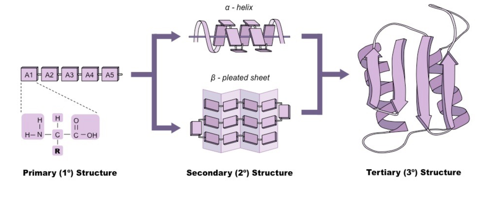
Figure 3. Protein structure: from amino acid sequences (1D) to alpha-helix, beta-sheet and random coil (2D) to all atom's representation (3D).
The Qian-Sejnowski Model
The Qian-Sejnowski protein 2D structure model is an example of a MLP with one hidden layer described in Figure 2.
Here is the code that implements the Qian-Sejnowski model.
Input layer
The inputs are sliding windows of 13 contiguous amino acids in the protein sequence. Each amino acid is described by a 21 one-hot encoding, for 20 amino acids and one more for a spacer. The spacer is used in training, where all training protein sequences are joined together connected by spacers.
We represent the input layer with \(x\) with dimensions \([N,I]\), where \(N\) is the number of total windows used in training, and \(I=13\) in this example.
Output Layer
For each input, the output is a 3-class softmax prediction for alpha helix (H) , beta sheet (B) or random coil (C).
\[H = [1,0,0]\\ B = [0,1,0]\\ C = [0,0,1]\]We represent the outputs with \(y\) with dimensions \([N,O]\), where \(N\) is the number of total windows used in training, and output dimension \(O=3\) is the three classifications of protein 2D structure.
Hidden layer
The hidden layer connects the input with the output layer. The variables of the hidden layer \(h\) have dimension \([N,H]\). The variables of the hidden layer are the outputs of the previous layer (the Input layer here), and the inputs of the next layer (the Output layer in this case).
The weights
The parameters of the models are two sets of weights and biases:
-
\(W^1[I,H]\) and \(b^1[H]\) connect the inputs to the hidden layer
-
\(W^2[H,O]\) and \(b^2[O]\) connect the hidden layer to the output
Network
The network is a MLP with one hidden layer, as the one described in Figure 4. In the Qian-Sejnowski model, the input dimension is 13, the hidden dimension is 40, and the output dimension is 3.
Instead of a RELU function (as in Figure 4), the Qian-Sejnowski model uses as activation function the linear logistic function
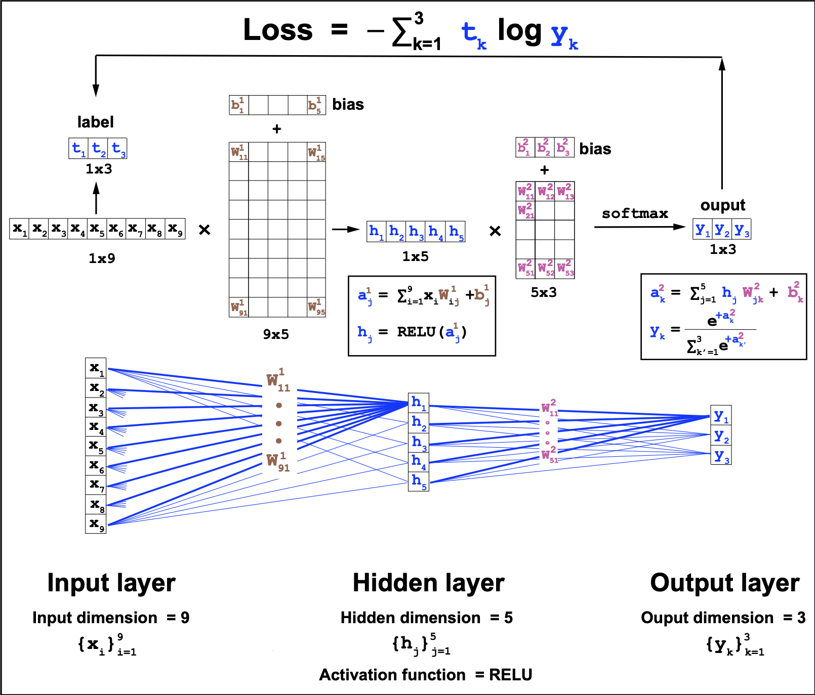
Figure 4. Multilayer perceptron with one hidden layer. This is a fully connected feed forward network. This particular MLP uses the RELU] logistic function. The input dimension of 9, the hidden layer dimension is 5, and the output dimension is a 3-class softmax.
The data
The data is a collection of protein sequences annotated with their secondary structure in the form of three states: alpha helix (H), beta strand (or sheet) (E) or random coil (C). Qian and Sejnowski used globin proteins. Here we are using the casp13, cb513 and ts115 datasets.
sliding one-hot windows
Each protein is split into 13 amino acid windows, moving one amino acid at the time. The inputs are all the 13 amino acid windows, and the output is a 3-class probability vectors describing the secondary structure (H, E or C) of the amino acid in the middle of the window.
The loss function
The loss function is the cross entropy between the true outcomes \((t^{(n)}_1,\ldots, t^{(n)}_O)\) and the predicted outcomes \((y^{(n)}_1,\ldots, y^{(n)}_O)\) summed to all \(1\leq n\leq N\) cases in the training set.
\[L(W^1, b^1, W^2, b^2) = - \frac{1}{N}\sum_{n=1}^N \sum_{o=1}^O t^{(n)}_o \log y^{(n)}_o.\]The predicted outcomes \(y^{(n)}_o\) depend on all the weight parameters \(W^1, b^1, W^2, b^2\) as described in Figure 4.
Training. Update of the parameters by stochastic gradient descent (SGD)
The parameters of the model are updated using stochastic gradient descent, that is the weights are updated iteratively (each iteration is called a epoch), and at each epoch, all the weights are modified by a quantity proportional to the negative loss change as a function of the parameters, that is, against the gradient or gradient descent
\[\begin{aligned} W^1_{ij} &\longleftarrow W^1_{ij} - \alpha \frac{\partial L}{\partial W^1_{ij}}\quad 1\leq i \leq I\\ b^1_{j} &\longleftarrow b^1_{j} - \alpha \frac{\partial L}{\partial b^1_{j}} \quad 1\leq j \leq H\\ W^2_{jk} &\longleftarrow W^2_{jk} - \alpha \frac{\partial L}{\partial W^2_{jk}}\quad 1\leq k \leq O\\ b^2_{k} &\longleftarrow b^2_{k} - \alpha \frac{\partial L}{\partial b^2_{k}}. \end{aligned}\]The meta-parameter \(\alpha>0\) is called the learning rate, and it is usually set to some small value such as \(0.1\).
The gradient descent process is not necessarily guarantee to converge to a minimum, but it often does. Results depend on many factor such as the learning rate, the database and the loss used. When you train a model, you watch the loss and how it decrease, and based on that, make a decision on when to stop the training and set on a value of the weight parameters.
Calculating the derivatives of the loss with respect to the different parameters is usually done by a method called backpropagation that we move to describe next in detail of our MLP with one fully connected hidden layer.
Backpropagation with one hidden layer
Because the Loss depends on all the parameters indirectly, calculating the derivatives of the Loss with respect to the parameters requires using the chain rule several times. That process is that in the field is referred to as backpropagation.
For this simple case of only one hidden layer, we are going to do the backpropagation explicit in the next section. Lucky for us PyTorch does the backpropagation for us. This is the code that implements the Qian-Sejnowski model both in python using explicit calculations of the gradients, and in PyTorch.
Using explicit calculations of the gradients
Using the notation introduced in Figure 4 for the 1 hidden layer MLP, we need to go backwards starting from the \(W^2\) and \(b^2\) weights. The Loss depends on those as
\[L \rightarrow y \rightarrow a^2 \rightarrow W^2, b^2\]we can write,
\[\begin{align} d W^2 := \frac{\partial L}{\partial W^2} &= \frac{\partial L}{\partial a^2} \frac{\partial a^2}{\partial W^2} = d a^2 \frac{\partial a^2}{\partial W^2}\\ d b^2 := \frac{\partial L}{\partial b^2} &= \frac{\partial L}{\partial a^2} \frac{\partial a^2}{\partial b^2} = d a^2 \frac{\partial a^2}{\partial b^2} \end{align}\]We leave for the appendix to show that for a the cross-entropy loss and \(y=\mbox{softmax}(a^2)\), then
\[da^2 := \frac{\partial L}{\partial a^2} = y - t.\]
Figure 5. Backpropagation for weights W2
Then
\[\begin{align} d W^2_{jk} &= \sum_{k^\prime} d a^2_{k^\prime} \frac{\partial a^2_{k^\prime}}{\partial W^2_{jk}} = d a^2_{k}\, h^1_j \\ d b^2_{k} &= \sum_{k^\prime} d a^2_{k^\prime} \frac{\partial a^2_{k^\prime}}{\partial b^2_{k}} = d a^2_{k} \end{align}\]In matrix notation:
- N = number of training examples
- I = input dimension
- H = hidden dimension
- O = output dimension
For \(W^1\) and \(b^1\), the dependencies are
\[L \rightarrow y \rightarrow a^2 \rightarrow h \rightarrow a^1 \rightarrow W^1, b^1\]then,
\[\begin{align} d W^1 := \frac{\partial L}{\partial W^1} = & \frac{\partial L}{\partial a^1} \frac{\partial a^1}{\partial W^1} = da^1 \frac{\partial a^1}{\partial W^1} = da^1 \cdot X\\ d b^1 := \frac{\partial L}{\partial b^1} = & \frac{\partial L}{\partial a^1} \frac{\partial a^1}{\partial b^1} = da^1 \frac{\partial a^1}{\partial b^1} = da^1\\ \end{align}\]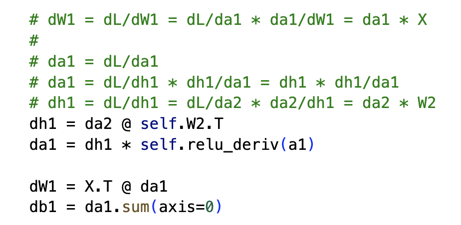
Figure 6. Backpropagation for weights W1
We use again the chain rule to calculate \(da^1\) as
\[da^1 := \frac{\partial L}{\partial a^1} = \frac{\partial L}{\partial h^1} \frac{\partial h^1}{\partial a^1} = d h^1 \cdot \frac{d\mbox{RELU}(a^1)}{d a^1}\]and \(dh^1\) can be calculated as a function of \(da^2\) as
\[dh^1 [N,H] := \frac{\partial L}{\partial h^1} = \frac{dL }{\partial a^2} \frac{\partial a^2}{ \partial h^1} = da^2[N,O] (W^2)^T[O,H]\]Finally,
\[dW^1 [I,H] = (X)^T[I,N] \cdot da^1 [N,H]\]Automatic backpropagation using PyTorch
The backpropagation calculation that we did for a MLP with one layer can be extended to more layer, but become very inefficient very quickly, specially considering that most models include large numbers of layers. PyTorch and other machine learning libraries become very practical as they are able to perform the backpropagation step to calculate all the parameters gradients automatically.
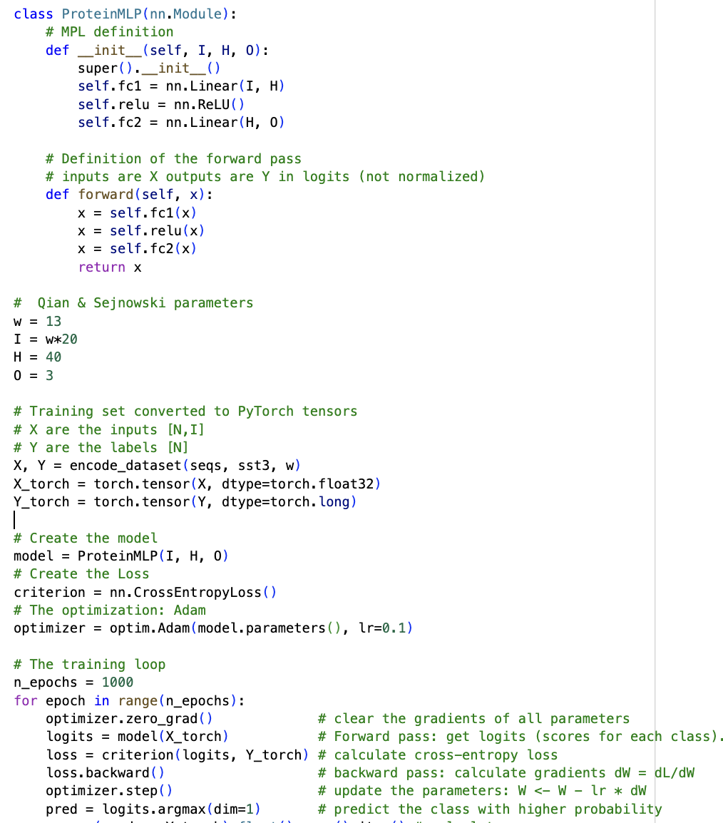
Figure 7. MLP with one hidden layer in PyTorch.
In PyTorch, one just needs to specify the Loss as a function of the weights and inputs, and it does the calculation of the gradients (vector of derivatives) automatically. As described in Figure 7, the steps are
- Define the MLP model: 1 hidden layer, RELU activation
- Sets dimensions: Input = I, Outputs = O, Hidden = H
- Assign Loss: CrossEntropyLoss
- Assign optimizer for parameter updates: Adam.
For 1000 epochs:
- Initialize optimizer
- Forward pass: get logits
- Compute cross-entropy loss
- Backpropagate gradients
- Update parameters
Here is the code that implements the Qian-Sejnowski model both in python using explicit calculations of the gradients, and in PyTorch.
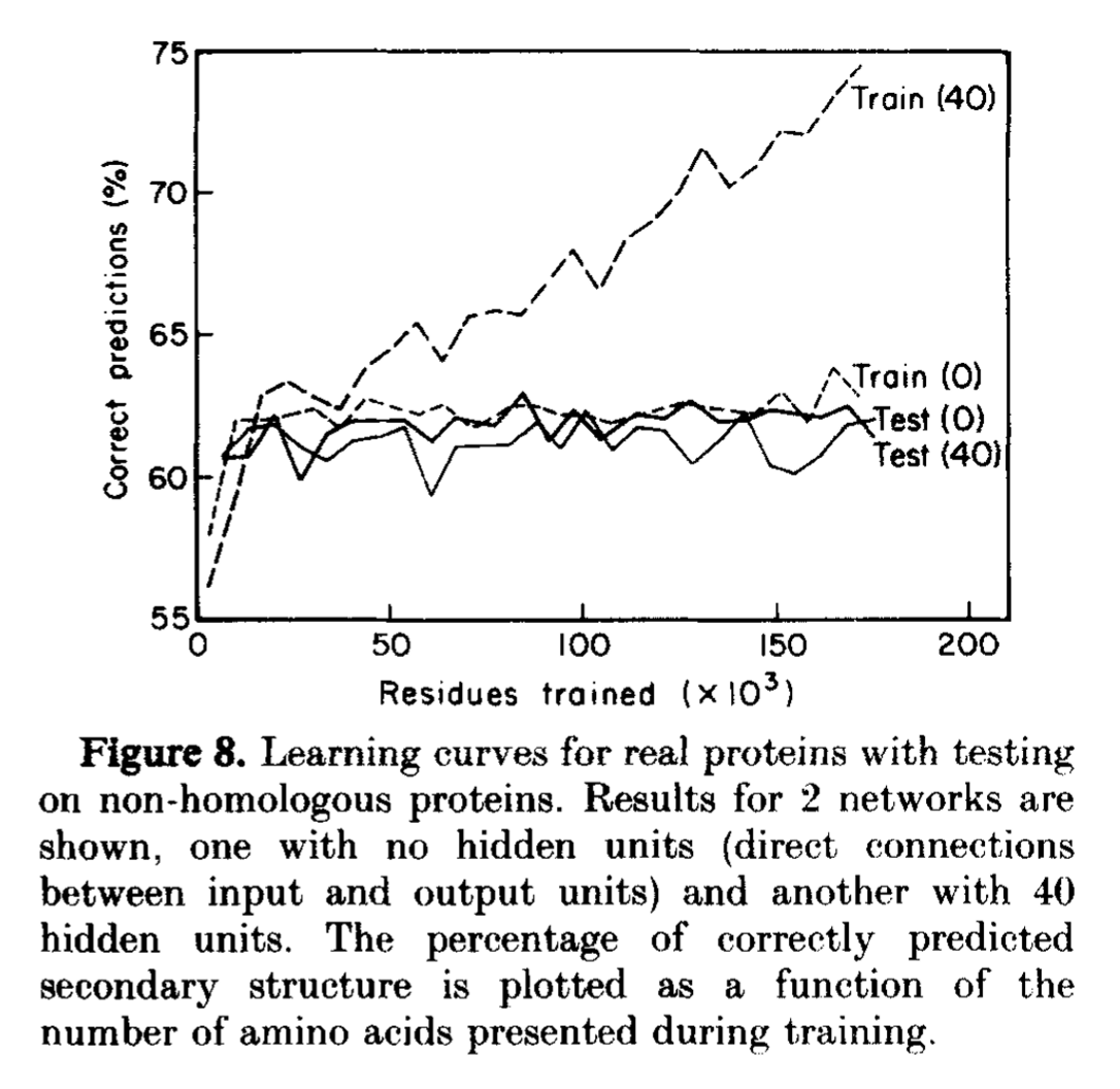
Figure 8. Figure from Qian & Sejnowski, 1988. Train(40) and test (40) results correspond to their 1 layer MLP with dimension 40 for the hidden layer. Train(0)/Test(0) are results using a perceptron with no hidden layers.
Overfitting
This paper already introduces the concept of overfitting. Overfitting refers to the fact that as models have more and more parameters, they become better and better to fit the parameters to the training date, to the point that those parameters do not perform well on a new example input that has not been seen in the training set before.
In the Qian-Sejnowski, they are careful train their model on one set of globing sequence, and they test on a different set of globins that has no sequence similarity (homologs) to the training set. See Figure 8 of paper reproduced here. Notice how the performance of test(40) is much lower than that of the training set train(40).
Fundamentals of neural networks
Figure 9 describe some of the basic elements of most deep learning methods.
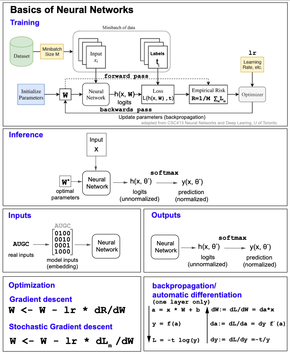
Figure 9. Fundamentals of neural networks.
Training
The basic elements of training are
The training set
The dataset used for training the parameters which includes the inputs (\(x\)) and labels (\(t\)) used for supervised learning.
Minibatch
To include randomness in the process, not all the training examples are used at once, at each training iteration only a subset of the training examples are used in te gradient descent optimization of the weight, (a minibatch).
Examples for each minibatch are sampled from the training data without replacement. A epoch (epoch) consists of a number of minibatch parameter update steps such that all training examples have been considered.
For instance, if the training set has 20,000 examples, and we choose a batch size of 100, then each minibatch has 100 examples and a epoch will consist of 200 minibatch updates (20,000/100)
There is usually a trade-off between the size of the batch size, the accuracy of the optimization and generalization. As the minibatch size increases, the accuracy of the gradients also increases, but the accuracy of the model predicting previously unseen cases (generalization) may decrease.
Weights’ initialization
The weights of the model are usually initialized to random numbers at the start of the training process. It is important to be aware that different initializations may affect the gradients and the optimization process. Also, weights should not be initialized to very large of very small values, as that may result in exploding gradients or vanishing gradients respectively.
Most Deep learning frameworks (like PyTorch) have standard initializations that they apply for different tipes of networks (Linear, CNN, transformer…) in combination with different activation functions (RELU, tanh, sigmoid…)
Optimization
The optimization of the parameters \(W\) is performed by minimizing a loss function which measures how the outputs of the network for the training set \(y_m\) are different from the labels \(t_m\).
\[W^\star =\mbox{argmin}_{W} L\left(y(x,W), t\right)\]It is standard to perform the parameter’s update towards a minimum by gradient descent, where the parameters are modified by a quantity proportional to the gradient of the loss.
The parameters at the next iteration \(k+1\) are given as a function of the parameters at the current \(k\) iteration as
\[W^{k+1} \leftarrow W^k - \alpha \frac{\partial L \left(y(W^{k})\right) }{\partial W}.\]The learning rate
The learning rate is the positive proportionality constant \(\alpha > 0\) between the change of the parameters and the loss gradient. The learning rate should not be to large (the gradients will blow up) or too small (changes are too small and it takes for ever to converge).
It is quite frequent and standard to use for automatic optimization a method called Adam, which is a refinement of the expression above. In Adam optimization, instead of a fixed learning rate \(\alpha\), there is a learning rate scheduler, such that the actual learning rate also changes at each epoch.
Backpropagation
Backpropagation is the name given to calculate the loss gradients respect to the parameters.
The loss does not depend explicitly from the weights, thus we need to apply the chain rule to backprogate the errors. This is also referred to as the backward pass.
As an example, for the case of a of a MLP with one hidden layer, backpropagation works as follows,
In the forward pass (left) given the inputs and weights, the outputs \(y\) and all intermediate values are calculated. Then, introducing the notation \(d v := \frac{\partial L}{\partial v}\), we can compute the gradients of loss wrt the weights by using those values in the backward pass (right).

Figure 10. Calculation of the derivatives computed directly from the values obtained by the forward pass (rather than as a mathematical operation). Notation: dv := dL/dv.
Using PyTorch once the model has been define and the loss has been calculated, the backpropagation step is done automatically simply declaring “loss.backward()”.
Inference
At inference, there are only inputs, but not labels. We use the best set of parameters previously trained by the model, and we use a forward pass to calculate the output of the model, which are the predictions.
Inputs
The inputs need to be converted into a numerical representation, or embedding. A typical embedding is a onehot. Other more complicated embedding could be the output of a language model.
Outputs
The outputs as they come out of the last layer of the model are usually unnormalized. In general, there is one final softmax conversion to convert them into a probability distribution amongst all possible outcomes.
The activation function
The activation function is a (usually nonlinear) function applied to a neuron’s input in a neural network to produce its output. Some examples of activation functions are sigmoid, tanh, ReLU, GeLU, and softmax (for an output layer).
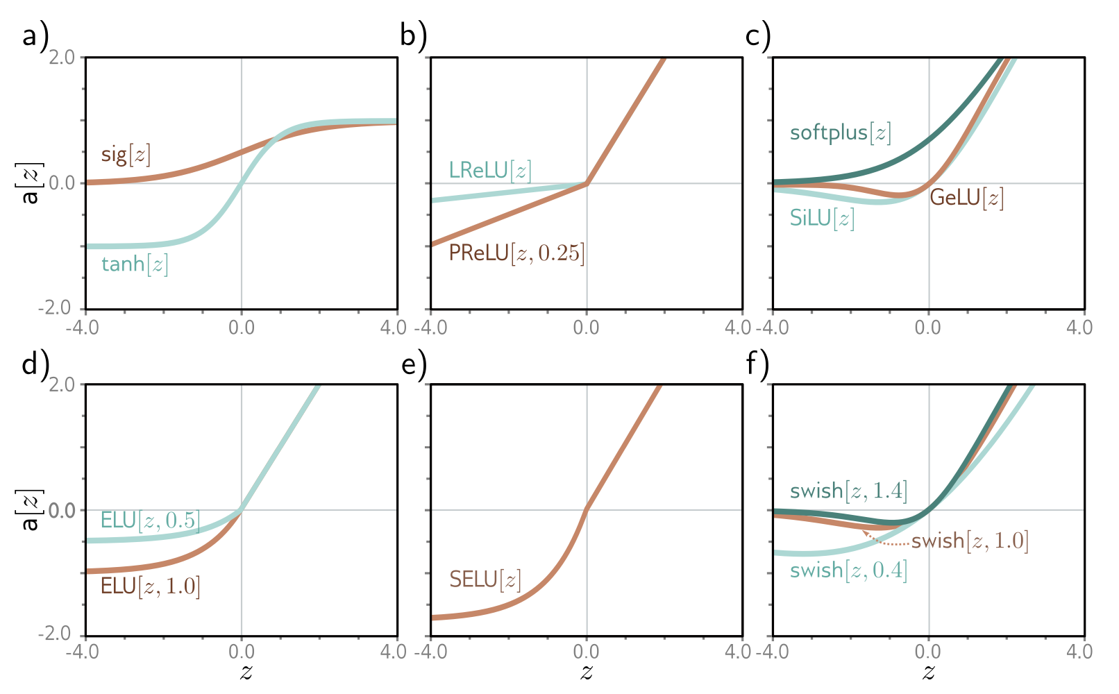
Figure 10. From "Understanding deep learning" Figure 3.13, different activation functions.
The Cross-entropy loss
Consider the case of a multi-class classification \(K\). For each input \(x[I]\), for instance the one-hot encoding of a 13-amino acid sequence (\(I=20\times 13=260\)), such that the number of classes is \(K\) (for instance \(K=3\) if the assignment is alpha-helix, beta sheet or random coil).
Then for each training example \(x[I]\), we assign a probability distribution \(t[K]\), that consists of all zeros but one value that is one. For instance,
\[\begin{aligned} x[I] \quad \sim \quad t[K] &= [1,0,0]\, \mbox{if}\, x\, \mbox{ is alpha helix},\\ x[I] \quad \sim \quad t[K] &= [0,1,0]\, \mbox{if}\, x\, \mbox{ is beta sheet},\\ x[I] \quad \sim \quad t[K] &= [0,0,1]\, \mbox{if}\, x\, \mbox{ is random coil}. \end{aligned}\]The output of the network, \(y[k](x, \theta)\) depends on the input \(x\) as well as the parameters (weights) of the model (\(theta\)).
The output of the network, \(y[k]\), can be converted into a probability distribution by softmax,
\[softmax(y)_k = \frac{e^{y_k}}{\sum_{k^\prime=1}^{K} e^{y_{k^\prime}}}\]Then for each example, we can now compare the two probability distributions \(t[K]\) to \(y[K](\theta)\). The KL divergence is a good method to compare two distributions. The KL divergence is non-negative, and it zero only when the two distributions are identical.
Thus a good way to define a loss for a categorical variable is to calculate the KL divergence
\[D_{Kl}(t||y) = \sum_{k=1}^K t_k \log\frac{t_k}{y_k},\]such that we would like to find the values of the parameters \(\theta\) that minimizes the KL divergence as,
\[\theta^* = argmin_{\theta} \sum_{k=1}^K t_k \log\frac{t_k}{y_k(\theta)}\]which can be re-written as
\[\begin{aligned} \theta^* &= argmin_{\theta} \sum_{k=1}^K t_k \log\frac{t_k}{y_k(\theta)}\\ &= argmin_{\theta} \left[ \sum_{k=1}^K t_k \log (t_k) - \sum_{k=1}^K t_k \log (y_k(\theta)) \right]\\ \end{aligned}\]And because \(t\) does not depend on the weights, we have
\[\begin{aligned} \theta^* &= argmin_{\theta} \left[ \sum_{k=1}^K t_k \log (t_k) - \sum_{k=1}^K t_k \log (y_k(\theta)) \right]\\ &= argmin_{\theta} \left[ - \sum_{k=1}^K t_k \log (y_k(\theta)) \right]. \end{aligned}\]The quantity
\[- \sum_{k=1}^K t_k \log (y_k(\theta))\]is defined as the cross entropy between \(t\) and \(y\).
We have shown that finding the parameters that minimize the cross entropy \(- \sum_{k=1}^K t_k \log (y_k(\theta))\) is equivalent to finding the optimal parameters that minimize the difference between the two distributions \(t\) and \(y\).
Fitting the models
The optimization of the parameters is usual performed using some flavor of a gradient descent method.
Gradient descent
In gradient descent, we have a training set of inputs/labels \(\{x_n, t_n\}_{n=1}^N\), and we seek parameters \(\theta\) that will bring the output of the networks \(y_n (x_n,\theta)\) as close as possible to \(t_n\).
The basic gradient descent algorithm, starts with some arbitrary values of the parameters \(\theta_0\), and
-
Calculate the derivative of the loss with respect to the parameters:
\[\frac{\delta L}{\delta \theta_i}\]where the loss includes the contribution of all data examples
\[L = \frac{1}{N} \sum_{ n= 1} ^N L_n(x_n, \theta)\] -
Update the weights moving against the direction of the change as
where the learning rate \(\alpha\) is a positive quantity.
Stochastic gradient descent
Stochastic gradient descent (SGD) is a flavor of gradient descent that introduces more randomness in the process by not considering all training examples in the calculation of the gradient.
Batches and epochs
In particular, it is standard to consider at each step of the gradient descent algorithm (iteration) to take a random subset of examples (a batch) in the training set to calculate the gradient as
\[\theta_i \leftarrow \theta_i - \alpha\, \sum_{m\in batch}\frac{\delta L_m}{\delta \theta_i}\]This introduces randomness in the gradient descent process.
The batches are usually drawn from the training examples without replacement. The algorithm works through the training examples until it has used all of them, at which point it starts sampling from the full training dataset again. A single pass through the entire training dataset is called an epoch. While the cases in each batch are selected at random, after each epoch, all training examples have been considered.
The batch size is arbitrary, and it can be anything from just one example to all of them. When all examples are used as a batch, that is the (non-stochastic) gradient descent again.
The number of steps in a epoch is equal to the number of total number of examples divided by the batch size.
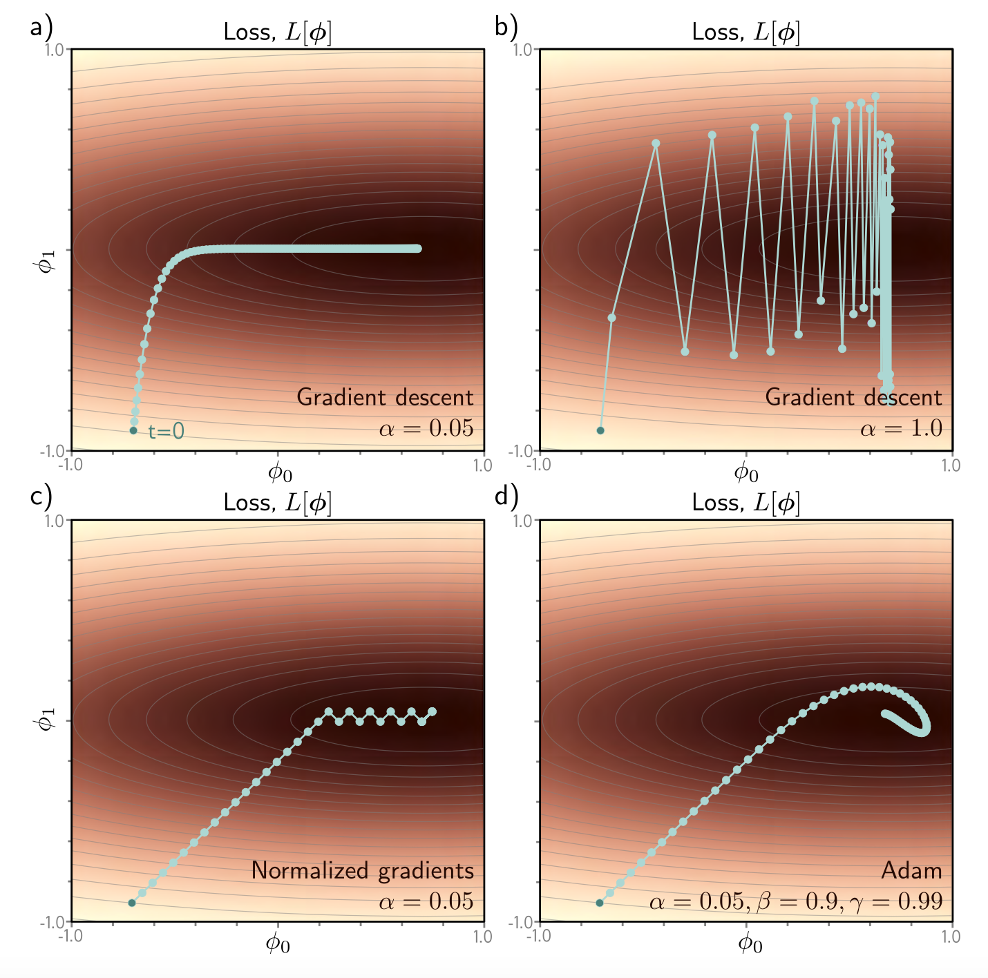
Figure 11. Comparison of different gradient descent methods. (Figure 6.9 from Understanding Deep Learning, Prince).
Adam (Adaptive momentum estimation)
Adam (Kingma & Ba, 2015) is a widely used method for stochastic optimization. As SGD introduced above, Adam only uses first order derivatives, but it estimates first and second order momentums of the gradients, and uses different learning rates for each of them.
The steps of the Adam stochastic optimization algorithm are, for a learning rate \(\alpha > 0\), and rates \(\beta_1, \beta_2\in [0,1)\),
- Get gradients at time t
- Update first momentum estimate
- Update second momentum estimate
-
Bias-correct first momentum
\[\hat{m_t} \leftarrow \frac{m_t}{1-\beta_1^t}\] -
Bias-corrected second momentum
\[\hat{v_t} \leftarrow \frac{v_t}{1-\beta_2^t}\] -
Update parameters
\[\theta_t \leftarrow \theta_{t-1} - \alpha \frac{\hat{m_t}}{\sqrt{\hat{v_t}} + \epsilon}\]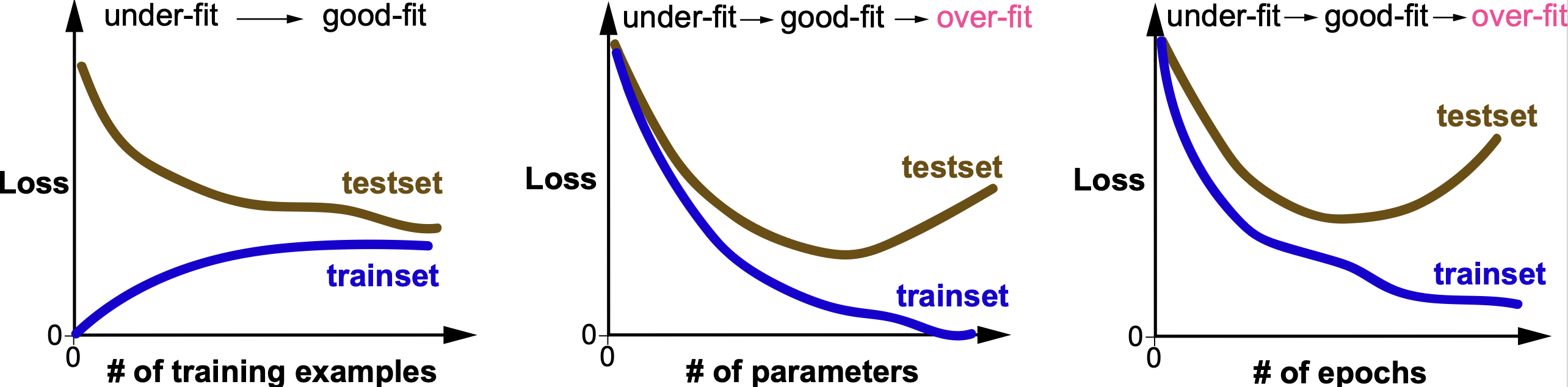
Figure 12. Training and Loss curves as a function of amount of training data, number of parameters and number of epochs used for training.
Generalization
The training of a neural network assures that the model fits well to the training data. But, how to make sure that the model also fits well to data that it has not seen yet but that it has also been drawn from the same data distribution?
This important questions is called generalization of the model. Generalization can be quite tricky.
As depicted in Figure 12, many factor can contribute to the generalization (or lack there off) of a given model. Some important ones are:
-
The amount of training data. More training data usually improves generalization
-
The number of parameters. Too few parameters results in underfitting (also referred to as high bias), and too many parameters tend to result in overfitting (also referred to as high variance)
-
The number of epochs used at training. For this variable, there is usually a sweet spot, such that often too many training epochs continue increasing the fit to the data to the expense of making the fit to the test data worse.
There are several well-establish techniques to improve generalization. But many lack strong theoretical grounding and are used mainly by trial and error. Some of those techniques are:
Adding more data
Reduction of parameters adding a bottleneck layer
Large weights induce overfitting
Regularization using \(L^2\) and \(L^1\) norm
Early stopping
Stochastic regularizations
-
Dropout
-
Noise injection
Appendix
Here we show that for the cross-entropy loss
\[L = - \sum_k t^k \log y^K\]such that the predictions \(y\) are a softmax,
\[y^k = \frac{\exp{a^k}}{\sum_{k^\prime} \exp{a^{k^\prime}}},\]and the labels \(t\) are one-hot encoded
\[\sum_k t_k = 1\]then
\[d a_k := \frac{\partial L}{\partial a^k} = y^k - t^k.\]Using the chain rule
\[d a^k := \frac{\partial L}{\partial a_k} = \sum_{k^\prime} \frac{\partial L}{\partial y_{k^\prime}} \frac{\partial y_{k^\prime}}{da_k}.\]We can see that
\[d y_{k^\prime} := \frac{\partial L}{\partial y_{k^\prime}} = - \frac{t_{k^\prime}}{y_{k^\prime}}\]Also
\[\frac{\partial y_{k^\prime}} {a_k} = \delta_{k {k^\prime}} y_{k^\prime} - y_k y_{k^\prime} = y_{k^\prime} \left(\delta_{k {k^\prime}} - y_k\right)\]thus,
\[\begin{align} \partial a^k &= \sum_{k^\prime} - \frac{t_{k^\prime}}{y_{k^\prime}} y_{k^\prime} \left(\delta_{k {k^\prime}} - y_k\right)\\ &= -\sum_{k^\prime} t_{k^\prime} \,\left(\delta_{k {k^\prime}} - y_k\right) = -t_k + y_k\,\sum_{k^\prime} t_{k^\prime} \\ &= y_k - t_k. \end{align}\]as the labels \(t[1,O]\) are one-hot encoded.