MCB128: AI in Molecular Biology (Spring 2026)
(Under construction)
(Now hiring TFs Fall 2026)
- Denoising Diffusion Probabilistic Models (DDPMs)
- The Diffusion encoder (forward process)
- The joint probability distribution \(q(z_{1:T}\mid x)\)
- Reversing the process? \(q(z_{t-1}\mid z_t)\)
- Other important diffusion probability distributions
- The Diffusion decoder (reverse/generative process)
- Diffusion Training by a variational upper bound
- Implementation:
- Denoising diffusion summary
- Diffusion models with self-conditioning.
- RoseTTAFold diffusion (RFdiffusion): de novo design of protein structures
- The diffusion forward process for translations and rotations (SE(3))
- The diffusion reverse process for translations and rotations
- Diffusion with Self-Conditioning
- The mean-squared error denoising loss
- Training and fine tuning
- Validation of RFdiffusion outputs using AF2
- SE(3) denoising diffusion models.
- Flow Matching Models
- The Virtual Cell
block 6: Diffusion Models & Protein design (RFdiffusion) / Graph Neural Networks
Denoising Diffusion Probabilistic Models (DDPMs)
The probabilistic interpretation of diffusion in deep learning that we are going to describe in this notes, comes from the manuscript Denoising Diffusion Probabilistic Models by Ho et al. We will also follow chapter 18 of the book UDL.
In a denoising diffusion model there is an encoder and a decoder. Figure 1 shows a high level description of a diffusion model. It consists of two parts: an encoder that introduces noise into the data, and a decoder that reverses the process to provide a probability distribution that allows to sample new examples from an approximation to the probability of the data. The encoder takes data \(x\), and transforms it in a series of successive steps \(z_1, \ldots z_T\) into noise data. The decoder then reverses the process one-by-one \(z_T, z_{T-1},\ldots z_1\) until it reproduces the input data \(x\).
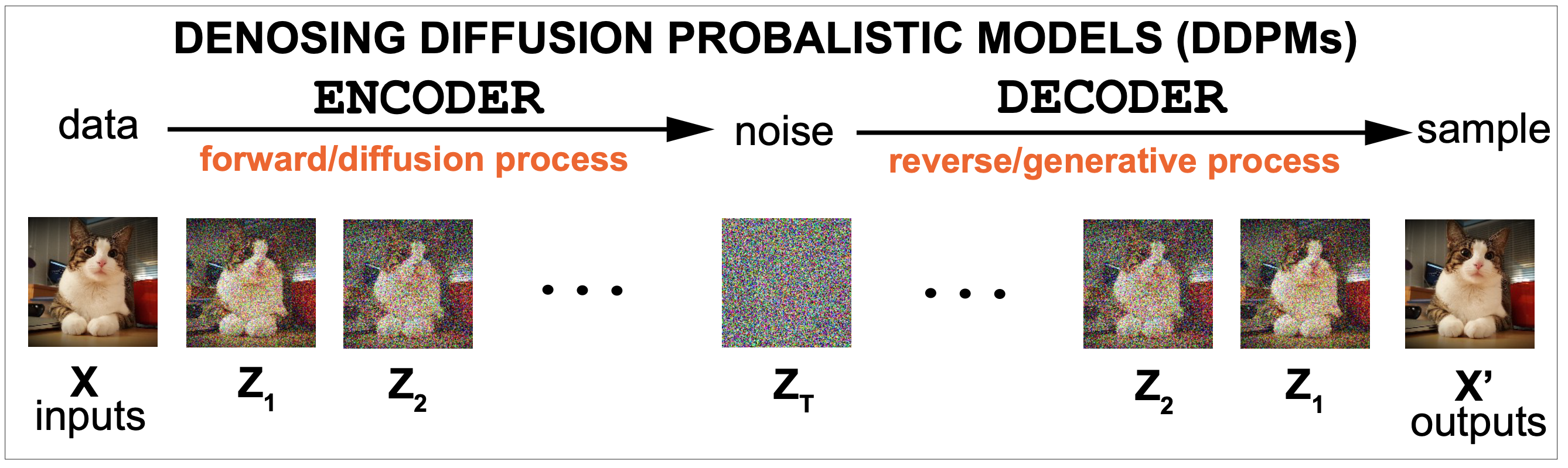
Figure 1.
Diffusion models are generative, which means in the process they learn a probability distribution from the data that can then be used to generate new examples.
Diffusion models are Markov processes. They involve an step-by-step (time) process of first adding noise, to then reverse it, in which the probabilities at a given time instance depend only on the variables at the previous time.
DDPMs use the variational principle to approximate the marginal probability of the data using a evidence lower bound (ELBO) to minimize.
Denoising diffusion can also be understood as score-base generative modeling with stochastic differential equations. Interpreting the Denoising Diffusion Markov chain as a process at infinitesimal times, one can derive differential equations describing the diffusion forward and generative processes. I am not going to describe this derivation here. The manuscript that introduced diffusions models using stochastic differential equations is this by Song et al, 2021. Part (2) in this google write up gives a very nice description of it as well.
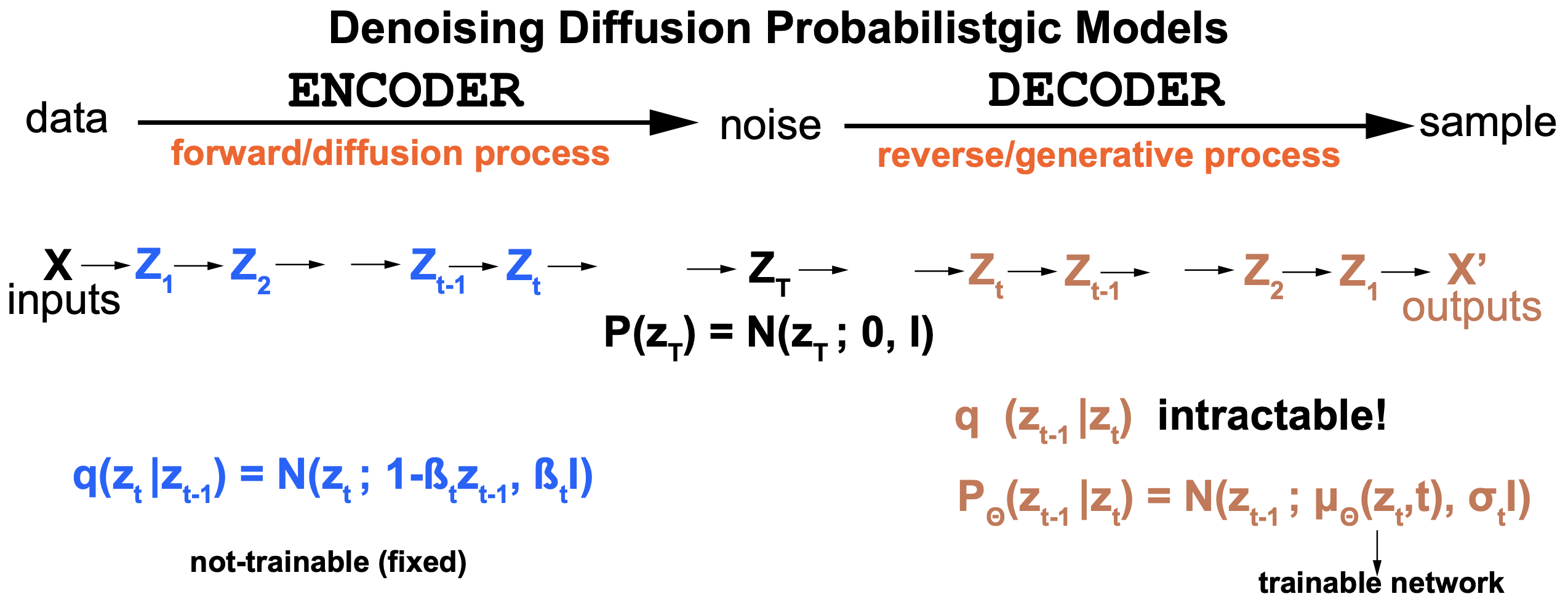
Figure 2. The two processes of the denoising diffusion models. Left (in blue) is the forward or diffusion process. Right (in brown) is the denoising generative process.
A diffusion model consist of an encoder and a decoder that we describe next.
The Diffusion encoder (forward process)
The diffusion or forward process is described in Figures 2 and 3.
The encoder of forward process takes the input data \(x\) and in a series of Markov steps it generates latent variables \(z_1, z_2,...\) adding Gaussian noise
\[\begin{aligned} z_1 = \sqrt{(1-\beta_1)}\, x + \sqrt{\beta_1}\epsilon_1\\ z_t = \sqrt{(1-\beta_t)}\, z_{t-1} + \sqrt{\beta_t}\epsilon_t\\ \end{aligned}\]where all the parameters, \(\beta_t\in [0,1], t=1...T\), are pre-specified values, and \(\epsilon_t\) are values sampled from the standard normal distribution.
In terms of probability distributions we have for the diffusion or forward process,
\[P(z_t\mid z_{t-1}) = N(z_t; \sqrt{(1-\beta_t)}\, z_{t-1}, \beta_t I)\]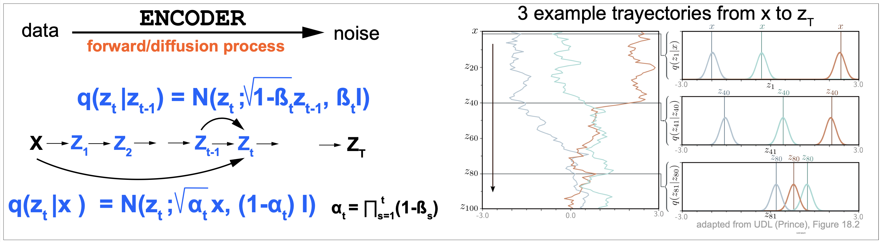
Figure 3. The forward or diffusion process.
As described in Figure 3 (right), starting from a data point, the latent variables first dampen the value by the quantity \(\sqrt{1-\beta_t}\), and then they add a Gaussian noise of mean zero and variance \(\beta_t\). After a number of iterations, the latent variable becomes almost indistinguishable from a sample from the standard normal distribution.
The joint probability distribution \(q(z_{1:T}\mid x)\)
Because of the Markov property of the model, we have for the join probability distribution of all latent variables
\[q(z_{1:T}\mid x) = q(z_1\mid x) \prod_{t=2}^T q(z_t\mid z_{t-1}).\]Reversing the process? \(q(z_{t-1}\mid z_t)\)
\[q(z_{t-1}\mid z_t)\]is the quantity that we would like to use to de-noise the process and generate new images or structures, however this “posterior” distribution is in most cases intractable. The reason is that it
In order to write this posterior distribution in terms of the forward distribution that we know \(q(z_{t}\mid z_{t-1})\) using Bayes theorem as,
\[q(z_{t-1}\mid z_t) = \frac{q(z_{t}\mid z_{t-1}) q(z_{t-1})}{q(z_t)}\]however we do not now the marginal distributions, and to calculate them, which we could using the join distribution \(q(z_{1:T} \mid x)\) and the expression
\[q(z_t) = \sum_{z_1,...,z_{t-1},z_{t+1},...,z_T} q(z_{1:T} \mid x)\]is usually intractable due to computing complexity.
Other important diffusion probability distributions
Diffusion kernel \(q(z_t\mid x)\)
We can directly add noise from the data to an arbitrary time step \(t\) because there is a nice close-form expression of the probability distribution
\[P(z_t\mid x) = N(z_t; \sqrt{\alpha_t}\, x, (1-\alpha_t)\, I)\]for \(\alpha_t = \prod_{s=1}^t (1-\beta_s)\).
That is, a sample \(z_t\) at time \(t\) can be obtained directly from \(x\), by simply sampling an \(\epsilon\) from the standard normal distribution as
\[z_t = \sqrt{\alpha_t}\, x + \epsilon\, {\sqrt(1-\alpha_t)}.\]UDL Section 18.2.1 has a detailed derivation of this result
Conditional diffusion distribution \(q(z_{t-1}\mid z_t x)\)
We cannot calculate the posterior denoising probabilities \(q(z_{t-1}\mid z_t)\) directly because we don’t know the marginal distribution of the latent variable \(q(z_{t-1})\). However, when the data \(x\) is known, then we know \(q(z_{t-1}\mid x)\). Thus it is possible to reach an analytic expression for \(q(z_{t-1}\mid z_t, x)\).
UDL Section 18.2.4 has a detailed derivation, and here we reproduce the result.
\[q(z_{t-1}\mid z_t, x) = N(z_{t-1}; \mu_t(z_t,x), \frac{\beta_t (1-\alpha_{t-1})}{\alpha_t} I)\]where
\[\mu_t(z_t,x) = \frac{1-\alpha_{t-1}}{1-\alpha_t}\,\sqrt{(1-\beta_t})\, z_t + \frac{\sqrt{\alpha_{t-1}}\,\beta_t}{1-\alpha_t}\, x.\]This distribution is important as it is going to appear in the calculation of the loss function. Also, our diffusion method of interest RFdiffusion uses it in some interesting ways, as we will see later.
The Diffusion decoder (reverse/generative process)
The true reverse denoising distribution is \(q(z_{t-1}\mid z_t)\) given by
\[q(z_{t-1}\mid z_t) = \frac{q(z_{t}\mid z_{t-1}) q(z_{t-1})}{q(z_t)}\]This distribution is usually intractable, and in the decoder we approximate it by a Normal distribution \(P_{\theta}(z_{t-1}\mid z_t)\) which depends on parameters \(\theta\). The approximation by a Normal distribution is appropriate for small values of \(\beta_t\).
\[p_{\theta}(z_{t-1}\mid z_t) = N(z_{t-1}; \mu_{\theta}(z_t,t), I)\]where the Normal distribution’s mean \(\mu_{\theta}(z_t,t)\) is trained by some deep learning method.
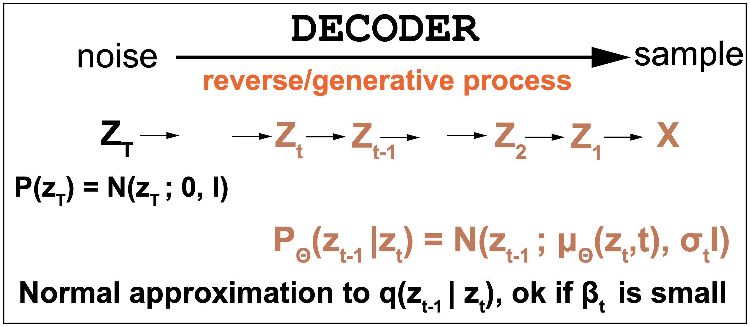
Figure 4. Generative denoising model.
The marginal probability of the data \(p_{\theta}(x)\)
The join probability of the data and latent variables is given by
\[p_{\theta}(x,z_{1:T}) = p_{\theta}(x\mid z_1)\, \prod_{t=2}^T p_{\theta}(z_{t-1}\mid z_t)\, p(z_T)\]The marginal probability of the data is found by marginalizing all latent variables as
\[p_{\theta}(x) = \sum_{z_1:T} p_{\theta}(x,z_{1:T})\]Diffusion Training by a variational upper bound
To train the model we want to maximizing the log probability of the data with respect to the parameters \(\theta\),
\[\theta^\star = argmax_{\theta} \sum_{i=1}^I\log p_{\theta}(x_i)\]This quantity is too difficult to calculate in general, so similar to variational autoencoders, we are going to use an upper bound as follows.
\[\begin{aligned} -\log p_{\theta}(x) &= \sum_{z_{1:T}} \log p_{\theta}(x, z_{1:T}))\\ &=-\sum_{z_{1:T}} \log\left[q(z_{1:T}\mid x)\, \frac{p_{\theta}(x, z_{1:t}))}{q(z_{1:T}\mid x)}\right]\\ &\leq -\sum_{z_{1:T}} q(z_{1:T}\mid x)\,\log\left[\frac{p_{\theta}(x, z_{1:t}))}{q(z_{1:T}\mid x)}\right]\\ &= L_{\theta} \end{aligned}\]where we have used Jessen’s inequality.
This optimization of the loss has two objectives
-
(1) To make the approximate posterior \(p_{\theta}(z_{t-1}\mid z_t)\) as close as possible to the actual posterior \(q(z_{t-1}\mid z_t)\).
-
(2) To maximize the marginal probability of the data.
In a VAE these two roles are distributed between the encoder and the decoder. In a diffusion model both tasks are approached by the decoder which is the only one with trainable parameters.
The Diffusion Loss function
The loss L can be simplified into an expression that depends on the tractable posteriors \(q(z_{t-1}\mid z_t,x)\), and the approximate posteriors \(p_{\theta}(z_{t-1}\mid z_t)\).
The final expression introduced by Ho et al. 2020 is given by
\[L = D_{KL}\left( q(z_T|x) || p(z_T)\right) + \sum_{t>1} D_{KL}\left(q(z_{t-1}\mid z_t\, x) || p_{\theta}(z_{t-1}\mid z_t)\right) - log p_{\theta}(x\mid z_1)\]Because both distributions are Normal distributions, the KL divergence has a close form such that
\[\begin{aligned} L_t &=: D_{KL}\left(q(z_{t-1}\mid z_t\, x) || p_{\theta}(z_{t-1}\mid z_t)\right)\\ &= E_q \left[ \frac{1}{2\sigma_t^2}|| \mu_t(z_t, x) - \mu_{\theta}(z_t,t) ||^2 + C \right] \end{aligned}\]Reparameterization
The above expression for the loss can be furthe simplifies by taking into account that \(x\) can be rewrite as the diffuse latent \(z_t\) minus the noise added to it at
\[x = \frac{1}{\sqrt{\alpha_t}}\, z_t - \frac{\sqrt{1-\alpha_t}}{\sqrt{\alpha_t}} \epsilon\]and replacing that expression for \(x\) in the definition of \(\mu_t(z_t,x)\)
\[\mu_t(z_t,x) = \frac{1-\alpha_{t-1}}{1-\alpha_t}\,\sqrt{(1-\beta_t})\, z_t + \frac{\sqrt{\alpha_{t-1}}\,\beta_t}{1-\alpha_t}\, x.\]results in the simplified expression
\[\mu_t(z_t,\epsilon_t) = \frac{1}{\sqrt{(1-\beta_t)}}\, z_t - \frac{\beta_t}{\sqrt{(1-\alpha_t)}\,\sqrt{(1-\beta_t)}}\, \epsilon_t\]A full derivation of this results can be found in UDL Section 18.15.1.
This results suggests a reparameterization of the denoising neural net such that it gets replaced with a different neural network to calculate the noise \(\epsilon_{\theta}(z_t)\) as
\[\mu_{\theta}(z_t,x) = \frac{1}{\sqrt{(1-\beta_t)}}\, z_t - \frac{\beta_t}{\sqrt{(1-\alpha_t)}\,\sqrt{(1-\beta_t)}}\, \epsilon_{\theta}(z_t)\]With this reparemeterization the loss becomes
\[\begin{aligned} L_t &= E_q \left[ \frac{\beta_t^2}{2\sigma_t^2\,(1-\beta_t)\,(1-\alpha_t)}\,|| \epsilon - \epsilon_{\theta}(z_t,t) ||^2 + C \right]\\ &= E_q \left[ \frac{\beta_t^2}{2\sigma_t^2\,(1-\beta_t)\,(1-\alpha_t)}\,|| \epsilon - \epsilon_{\theta}(\sqrt{\alpha_t}\,x+\sqrt{(1-\alpha_t)}\,\epsilon,t) ||^2 + C \right]\\ \end{aligned}\]which can be simmplified by removing the C constant (does not depeno on the parameters, and by using the simplification of setting the time-dependent coefficient to one,
\[\frac{\beta_t^2}{2\sigma_t^2\,(1-\beta_t)\,(1-\alpha_t)} = 1,\]as it was observed in Ho et atl, 2020 that otherwise the coefficient could get very large.
Then resulting in the loss is a simple minimum squared error (mse) between the applied noise \(\epsilon\) and the predicted noise at time \(t\),
\[\begin{aligned} L_t &= E_q \left[ || \epsilon - \epsilon_{\theta}(z_t,t) ||^2 \right]\\ &= E_q \left[ || \epsilon - \epsilon_{\theta}(\sqrt{\alpha_t}\,x+\sqrt{(1-\alpha_t)}\,\epsilon,t) ||^2 \right]\\ \end{aligned}\]Implementation:
Training
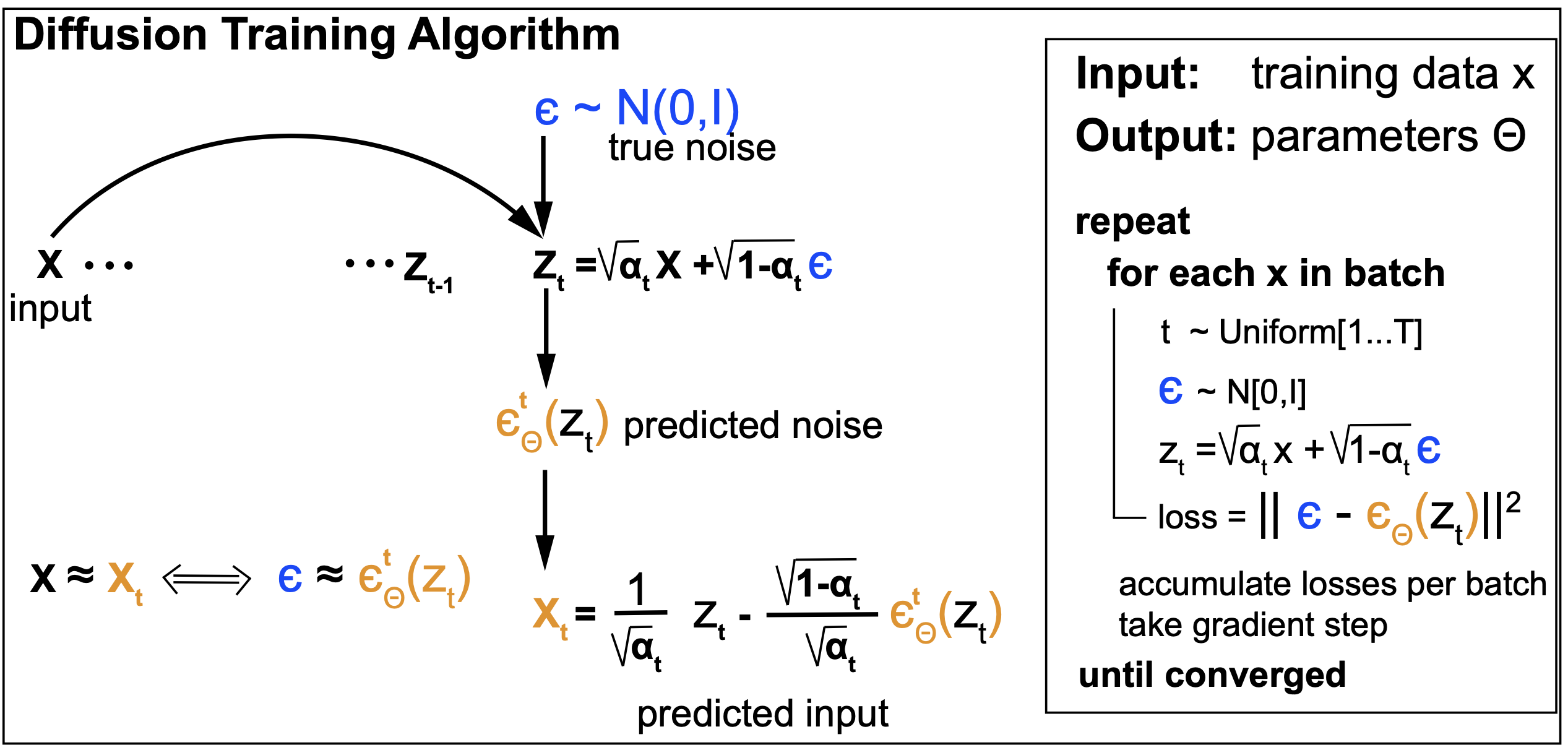
Figure 5.
Sampling
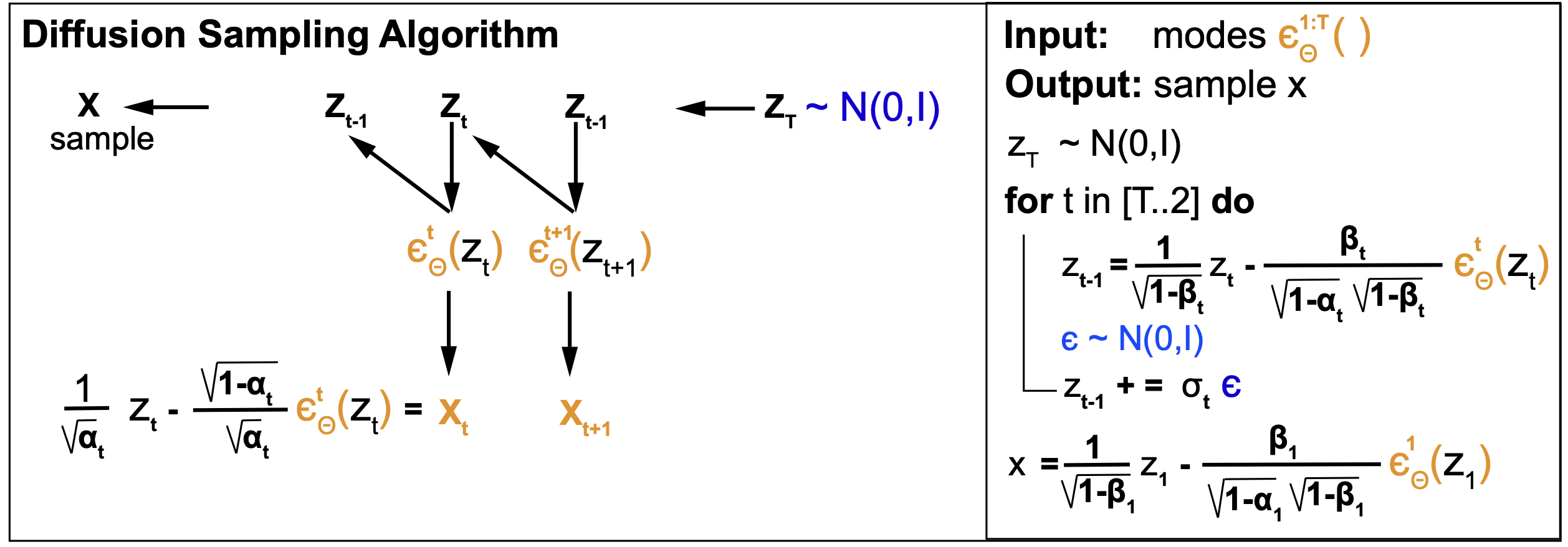
Figure 6.
Denoising diffusion summary
-
The input data is transformed in a Markov repeated process that successively adds Gaussian noise to the input data. This is the Encoder or forward process
-
Each step \(t\) defines a latent variable \(z_t\) that adds noise to the previous latent variable \(z_{t-1}\).
-
After a number of steps \(T\), the input \(x\) is degraded to random Gaussian noise \(z_T\).
-
The Forward process is stochastic and does not depend on any trainable parameter.
-
The reverse de-noising process is called the decoder or generative process. Reversing the diffusion process exactly is too hard.
-
The DDPM method approximates the decoding process by another Markov chain of Gaussian probability distributions. The mean of these Gaussian distributions are predicted each by a Deep Neural Network.
-
If the noising steps are sufficiently small, that justifies using Gaussian probability distributions to model the de-noising process.
-
The loss function, as in variational autoencoders, is based on the Evidence Lower Bound (ELBO).
-
After all is set and done, the loss function becomes a simple, efficient and easy to implement least-squares formulation.
Diffusion models with self-conditioning.
Self-conditioning was introduced in ChenZhangHinton, 2023. We discuss it here as RFDiffusion does use self-conditioning as well.
RoseTTAFold diffusion (RFdiffusion): de novo design of protein structures
We will study the method RFdiffusion (RFdiffusion supplemental materials) as our practical application of a diffusion model in molecular biology. RFdiffusion addresses the task of designing new protein folds from known existing folds.

Figure xx. RFDiffusion is a DDPM to generate new protein folds.
Denoising diffusion models were originally implemented to create images. Here
-
The “image” is a protein 3D structure.
-
The noise is applied to the reference frames of the backbone of each amino acid, starting from a real 3D protein structure.
-
The decoder (de-noiser) is the method RoseTTAFold, an already pretrained model for protein 3D structure prediction. Similarly to AlphaFold2 (AF2), RoseTTAFold (RF) moves reference frames (one for each amino acid) from an arbitrary origin to their locations in the 3D structure.
The diffusion forward process for translations and rotations (SE(3))
The diffusion reverse process for translations and rotations
Diffusion with Self-Conditioning
Introduced by Chen et al, 2023, Self-Conditioning
The mean-squared error denoising loss
Training and fine tuning
Validation of RFdiffusion outputs using AF2
SE(3) denoising diffusion models.
RFdiffusion is a diffusion model to generate novel protein folds. RFdiffusion applies diffusion to the reference frames N-C_alpha_N associated to each amino acid, similar to those used by AF2. RFdiffusion requires to use a RoseTTAFold (RF) model pretrained on protein structures. RFdiffusion also uses a heuristic loss. If you want to learn more principled diffusion models for SE(3) translations and translations, you want to read this manuscript by Yim et al, 2023.
Flow Matching Models
This section is still under construction. Follow the slides for more information.
We will discuss the basics of Flow Matching models and do an in-depth comparison to Denosing Diffusion models, since they share many elements, and they are alternative models for similar data generation problems.
We will discuss the work of the following manuscripts of different version of Flow Matching:
-
Flow Matching by Lipman et al, 2023.
-
Discrete Flow Matching by Gat et al, 2023.
Our practical application by Rubin et al, 2025 applies standard and discrete Flow Matching together to the question of generating new RNA sequences and structures.
The Virtual Cell
This section is still under construction. Follow the slides for more information.
We will discuss the following manuscripts
-
“The virtual Cell” by Tang, 2025
-
“How to build the virtual cell with artificial intelligence: Priorities and opportunities” by Bunne et al, 2024
-
“Towards multimodal foundation models in molecular cell biology” by Cui et al, 2025
-
“Calling all data” by Nat Meth editorial, 2025