MCB128: AI in Molecular Biology (Spring 2026)
(Under construction)
(Now hiring TFs Fall 2026)
- Language models
- Large Language models (LLMs)
- LLMs in genomics
block 4: Large Language Models (LLMs)/ LLMs for genomics and proteins
Pytorch code to implement the main methods described in the block, that is transformer-based encoders, decoders and encoder-decoders, can be found here.
Language models
A language model were originally designed to process and understand human language, and as a result of that to be able to generate new speech as well.
The idea of a “language” has been extended also to understand biological sequences, and we also talk about the language of DNA, the language of RNA, or the language of genes, amongst others.
Noam Chomsky pioneered work on language models in the 1950s, and introduced a hierarchical formalism of formal grammars to describe different types of languages with increasing complexity. Chomsky introduced a hierarchy of formal grammars: regular grammars, context-free grammars (CFGs), context-sensitive grammars and unrestricted grammars. The assumptions of most biological sequence algorithms correspond to those of regular grammars. For instance, hidden Markov models (HMMs), which are probabilistic regular grammars and we will briefly discuss next, used extensively for protein and DNA homology are regular grammars. And SCFGs which are probabilistic (stochastic) context-free grammars are used to describe RNA structure.
LMs are probabilistic (generative) models
The term Language Models (LMs) is used to describe probabilistic models which are able to generate new examples (sentences) of the language they represent. There is an underlying \(P_{data}\) that the LM tries to approximate by a \(P_{\theta}\) probability distribution, depending on a set number of parameters \(\theta\)
The LM gives a parametric representation of the data, where the data could be an actual natural language, or images of a particular object (dogs), or in our case of interest biological sequences of different characteristics such as protein structural families or RNA structural families, amongst others.
Learning
Learning in nothing but finding the set of parameters \(\theta^\ast\) so that that \(P_{\theta^\ast}\) best approximates the data distribution \(P_{data}\).
Some of the most important aspects in learning the parameters are
-
What data to use as representative for the language we are trying to model.
-
What objective function to use to compare the data and the parametric probability distributions.
-
What optimization procedure to use to minimize that objective function.
Inference
A trained generative model can be used for many purposes, some of the most obvious and important are
-
Density estimation: given a data point \(x\), to calculate its probability \(P_{\theta}(x)\) that it is belongs to the same language.
\[P_{\theta}(x)\]If we have trained a model to identify messenger RNAs (mRNAs), then we expect that
\[\begin{aligned} P_{\theta}(\mbox{AUG NNN NNN ... NNN UAA}) &= 0.01\\ P_{\theta}(\mbox{ UG NNN NNN ... NNN UAA}) &= 0.0000001 \quad \mbox{a deletion in the start codon AUG -> UG}\\ P_{\theta}(\mbox{AUG NNN NNN ... NNN UUA}) &= 0.00001 \quad \mbox{a mutation in the stop codon UAA->UUA}\\ P_{\theta}(\mbox{AUG NN NNN ... N UAA}) &= 0.001 \quad \mbox{a frameshift}\\ \end{aligned}\] -
Sampling: to generate novel data from the model distribution
\[x_{sample}=\, \sim\, P_{\theta}\]
Generative vs discriminative models
Discriminative models task is given a data point, to assign it a label. Generative models, on the other hand, describe a join probability distribution to describe both the data and their labels.
For instance a discriminative model for RNA structure will give you a structure “str” for an input sequence “seq”. A generative model of RNA structure (such as a SCFG) defines a distribution over sequences and structures. From an SCFG, you can sample RNA sequences with structures; and in general it allows to sample data examples with their labels.
-
Discriminative model: \(P(\mbox{str}\mid \mbox{seq})\)
-
Generative model: \(P(\mbox{str} ,\, \mbox{seq})\)
It is fair to say that a discriminative model also describe a probability (generative), that is the probability of all the possible labels (structures) given one data point (sequence). However the concept of generative model is usually reserved to models that can sample the whole data (sequences with structures).
The importance of sampling from a probability distribution
You may have noticed that the terms “generative (probabilistic) model” and “sampling” seem to come hand on hand.
Once you have a probability distribution over a set of random variables \(P(X,Y,Z)\), that results in the opportunity of taking samples from that distribution. Sampling values according to a probability distribution implies that values with higher probability will be sampled more often that values with very low probability. Any value is a possible sample, but for a large enough sample, the histogram of sampled values will resemble the shape of the probability distribution from where they were sampled. See Figure 1 for an example of the effect of the sample size.
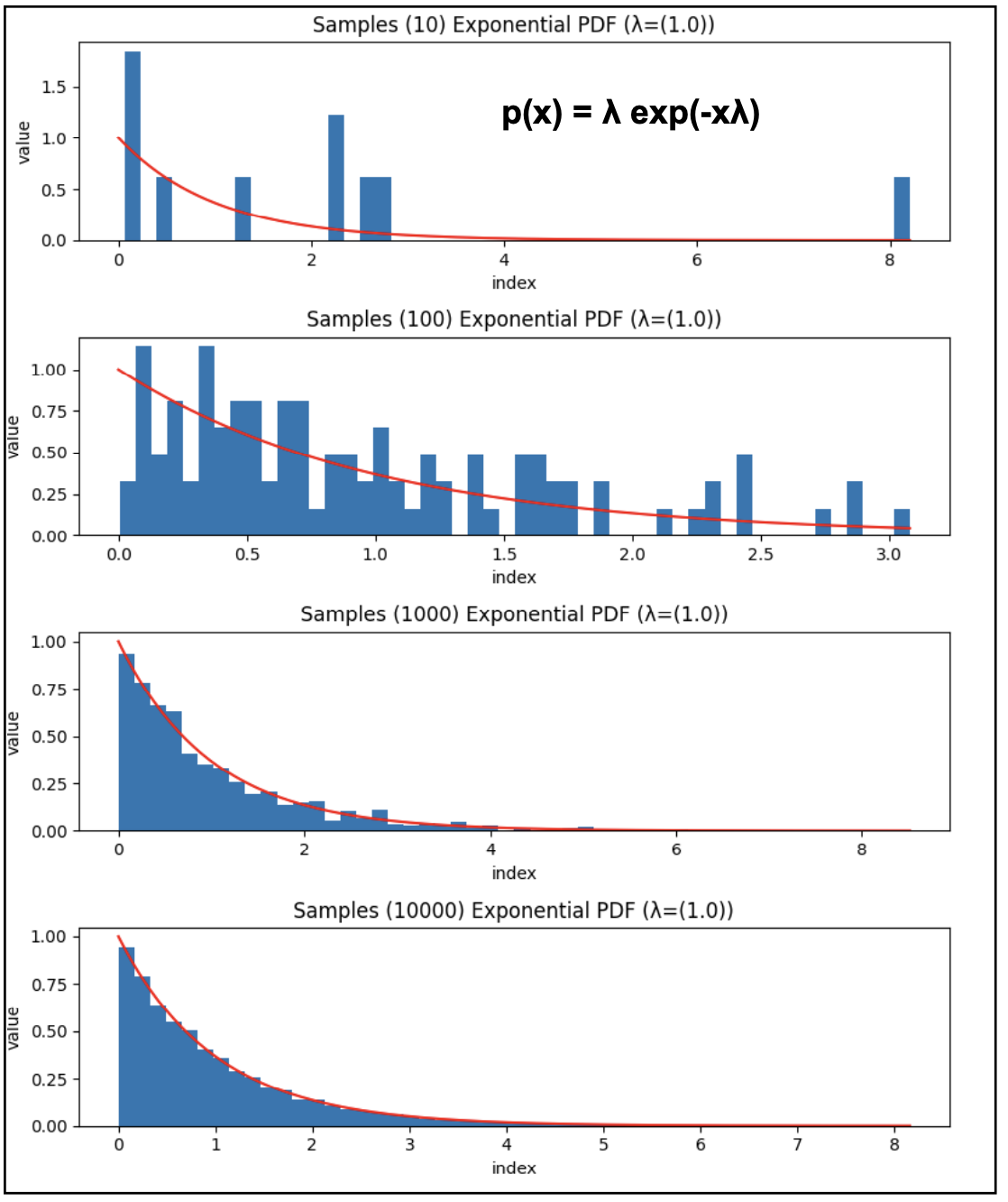
Figure 1. Samples 10, 100, 1000, 10000 from the exponential distribution with lambda = 1.0
Sampling is very often used to represent the whole distribution. Learning a joint probability distributions, specially when many variables are involved with high dimensionality, may be an almost impossible task, but if by some approximate method, we can take a representative sample of the distribution \(\{x_i y_k z_j\}_{i,j,k=1,1,1}^{N_x, N_y, N_Z}\),
then arbitrary quantities \(f\) over the probability distribution can be estimated using that sample as
\[<f(X Y X)> =: \int_{x,y,z} f(x y z)\, P(x y z) \approx \frac{1}{N_x N_y N_z}\, \sum_{i,j,k} f(x_i y_j z_k)\]This kind of approximation is usually referred to as Monte Carlo sampling.
Grammar-based LMs
Before we get into Transformer large language models (LMMs), we are going to consider two cases of grammar-based language models what have been very successful in molecular biology.
These LMs by being based on a grammar, the grammar already proposes an underlying structure for the language they are trying to describe. In contrast, LLMs are much looser, and one would expect to discover an underlying structure when trained on data from a particular language.
Grammar-based LMs can be trained by ML as there is a direct association between data labels and parameters, on the other hand with the transformer LMs, you need to propose an optimization procedure
Example1: hidden Markov models (to generate protein sequences)
Hidden Markov models (HMMs) are probabilistic generative methods that generate a language that follows a particular type of grammar.
Hidden Markov models (HMMs) as even simpler than autoregressive models.
Example2: stochastic context-free grammars (to generate RNA sequences+structures)
Stochastic context-free grammars (SCFGs) are generative models that describe sentences in which there are palindromic relationships, in particular, they are used in molecular biology to describe RNA structure.
Large Language models (LLMs)
Useful LLMs are autoregressive
Predicting the join probability distribution of all the data \(\{x_i\}_{i=1}^{L}\) can be very complicated. However any joint probability distribution can be expressed with total generality as a product of conditional probabilities for any arbitrary ordering of the data \((x_1, x_2,\ldots x_L\}\)
\[\begin{aligned} P(x_1,\ldots x_L) &= P(x_1)\, P(x_2|x_1)\, P(x_3|x_1 x_2)\ldots P(x_L|x_1 x_2\ldots x_{L-1})\\ &=P(x_1)\prod_{i=2}^L P(x_i|x_1\ldots x_{i-1}) \end{aligned}\]Autoregressive generative models make use of that general property to their advantage to simplify the model by specifying each of those conditional as parameterized functions with a fixed number of parameters.
For instance we could assume that each the conditionals describe Gaussian noise as
\[P(x_i|x_1\ldots x_{i-1}) = N(\mu = x_1a_1 + \ldots + x_{i-1}a_{i-1},\, \sigma^2=\epsilon^2).\]Transformer-based Large Language models
Transformer based models come mostly in three types
-
decoder. A decoder predicts the next token in a sentence. GPT3 is an example of a decoder.
-
encoder. An encoder transforms an input embedding into an output embedding that can be used for a variety of tasks down the road. BERT and BERT-like models are encoders.
-
encoder-decoder. An encoder-decoder is used for sequence to sequence tasks where a sequence is transformed into a different one (for example in translation). The sequence-to-sequence transformer of “attention is all you need” is an example of an encoder-decoder.
Because of these functions as text generators (decoders), text classifiers (encoders) and text translators (encoder-decoders), and the large number of parameters they involve, these types of models are referred to as large language models or LLMs. These days, transformers are at the hearth of almost all LLMs.
We will also study several LLMs used in molecular biology, such as DNABERT, ESM-1b, ProGen2, and Evo.
decoder-only (autoregressive models)
A decoder model is autoregressive. That is, a decoder does not calculate the joint probability distribution \(P(x_1 \ldots x_L)\) directly as it’s goal is to calculate the probability of the next token \(x_i\) given the tokens before it,
\[p(x_i\mid x_1\ldots x_{i-1}).\]In Figure 2A we describe a decoder. Pytorch code to implement a transformer-based decoder can be found here.
In a decoder, the goal at training is to find parameters that maximize the log probability of all the residues under the autoregressive parameterization for the sequences in the training set. This objective is just a reformulation of the cross-entropy loss,
\[\mbox{max} \prod_i P(x_i\mid x_{1:i-1}) = \mbox{max} \left(\sum_i \log P(x_i\mid x_{1:i-1})\right) = \mbox{min} \left(\sum_i -\log P(x_i\mid x_{1:i-1})\right) = \mbox{min}\, Loss(x_{1:L})\]where
\[Loss(x_{1:L}) = - \left(\sum_i \log P(x_i\mid x_{1:i-1})\right).\]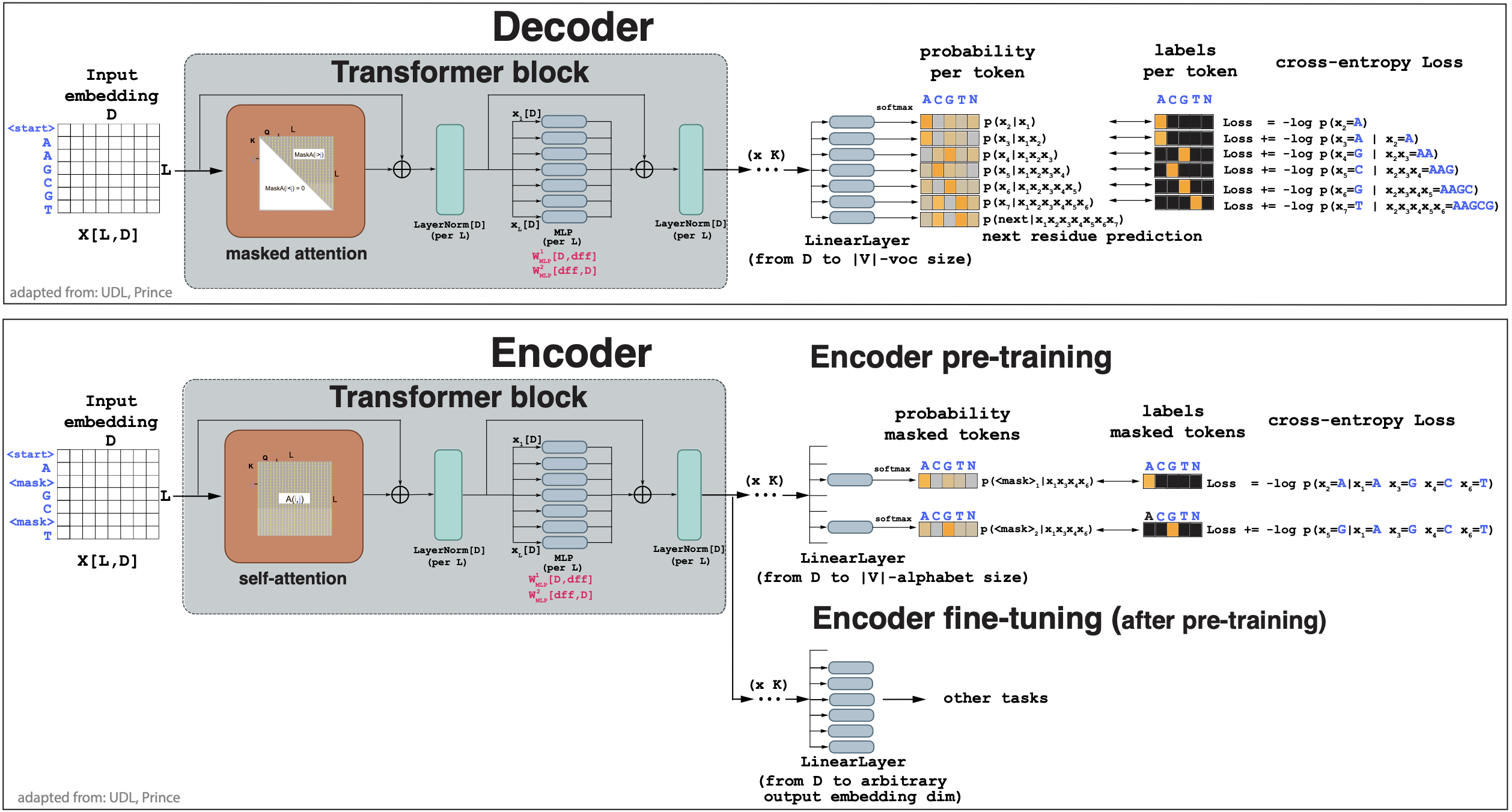
Figure 2. (A) A decoder network. Input is an embedding for a DNA sequence, output is a probability for each residue based on all residues before. (B) An encoder network. Input is an embedding for a DNA sequence with masked residues, output is a probability for the masked residues.
masked self-attention
The objective when training a decoder is to maximize the log probability of all tokens given only the tokens before it. In a transformer, the self-attention layers is the one responsible for the attention between tokens. In vanilla self-attention, all tokens interact with all other tokens. For the decoding task, we can achieve that by forcing that the attention to the right tokens is zero. This is referred to as masked self-attention.
Masked self-attention is very simply implemented adding a mask to the attention scores (before the softmaksing) such that
\[M(i,j) = \begin{cases} 0 & \mbox{if}\, i > j\\ -\infty & \mbox{if}\, i <= j \end{cases}\]then
\[masked-Attn(i,j) = \mbox{softmax}_k\left(\mbox{score}(q_i\dot k_j) + M_{ij}\right) = \begin{cases} \mbox{softmax}_k\left(\mbox{score}(q_i\dot k_j)\right) & \mbox{if}\, i > j\\ 0 & \mbox{if}\, i <= j\\ \end{cases}\]thus, masked attention is unchanged for \(i>j\) but there is no attention for tokens ahead \(i\leq j\).
The decoder autoregressive task guarantees that each residue contributes to the loss, but it has the limitation that it only considers the left context of each residue (or word). See figure 2A.
generating more tokens
Since the decoder provides as final output the probability of all tokens after a sentence has been seen, it allows to sample the next token. The sampled next token could be the one with the max probability or sample from that probability distribution. The new extended sequence could then be feed back to the decoder to generate another token. This is the fundamental mechanism of any chatbot.
decoder example: GPT3
GPT3 is a LLM that apply the decoder mechanism to large scale. Here are some numbers,
| vocabulary | V | 50,257 tokens |
| embedding | D | 12,288 |
| Transformer layers | K | 96 |
| Transformer heads per layer | h | 96 |
| query, key, value dimension per head | D_h | 128 |
| FF hidden dimension | d_ff | 49,152 |
| max length of input | Lmax | 2,048 tokens |
| training | words | 300 billion tokens |
encoder-only
The goal of an encoder is to learn some general information about the statistics of the language it is describing. We are going to consider encoders based on a transformer architecture, described in Figure 2A.
Pytorch code to implement a transformer-based encoder can be found here.
There are two phases in an encoder:
-
pre-training Using a large corpus of data the transformer is trained. The training method is self-supervision by masking some of the tokens in the inputs. In pre-training, data is not labeled.
-
fine-tuning. In this phase, the resulting network is adapted with some extra downstream layers to address some specific questions using a smaller body of labeled data.
encoder pre-training
In Figure 2A we describe a decoder. In a decoder, the goal at training is to find parameters that maximize the log probability of all the residues masked in the sequences in the training set. This objective is just a reformulation of the cross-entropy loss,
\[\mbox{max} \prod_{i\in mask} P(x_i\mid x_{\notin mask}) = \mbox{max} \left(\sum_{i\in mask} \log P(x_i\mid x_{\notin mask})\right) = -\mbox{min} \left(\sum_{i\in mask} \log P(x_i\mid x_{\notin mask})\right) = \mbox{min}\, Loss(x_{masked})\]where
\[Loss(x_{masked} = - \left(\sum_{i\in mask} \log P(x_i\mid x_{\notin mask})\right)\]Because the encoder pre-training does not require label data, just to mask tokens (residues), it is usually done in very large sets of data.
The encoder considers both left and right context for each residue (word), but it has the limitation that it does not make very efficient use of the data as only masked residues contribute to the loss.
encoder fine tuning for specific tasks
A pre-trained encoder produces an output embedding in some arbitrary dimension, that hopefully has captured statistical information about the language being learned (English or DNA). A pre-trained encoder later can be further trained (fine-tuned) for particular supervised tasks using much smaller datasets of labeled data.
encoder example: BERT
BERT stands for Bidirectional Encoder Representations from Transformers. BERT is a encoder-only model based on transformer layers as described in Figure 2B. BERT is meant to be trained in natural languages, mostly English, but there are many follow ups trained for different languages (or multilingual).
“Bidirectional” indicates that it is using a full attention block which explores attention from both left and right context (unlike decoders which by using masked attention only explore the left context).
The main specifications of BERT are
| vocabulary | V | 30,000 tokens |
| embedding | D | 1,024 |
| Transformer layers | K | 24 |
| Transformer heads per layer | h | 16 |
| query, key, value dimension per head | D_h | 64 |
| FF hidden dimension | d_ff | 4,096 |
| max length of input | Lmax | 512 tokens |
| pre-training | steps | 1,000,000 |
| pre-training | epochs | 50 |
| pre-training | words | 3.3 billions |
Some of the fine-tuning tasks explored by BERT are: sentence classification (positive, negative, informative…) or word classification (a place, a person, a verb…).
DNABERT is an almost direct reimplementation of BERT for DNA sequences that we discuss bellow.
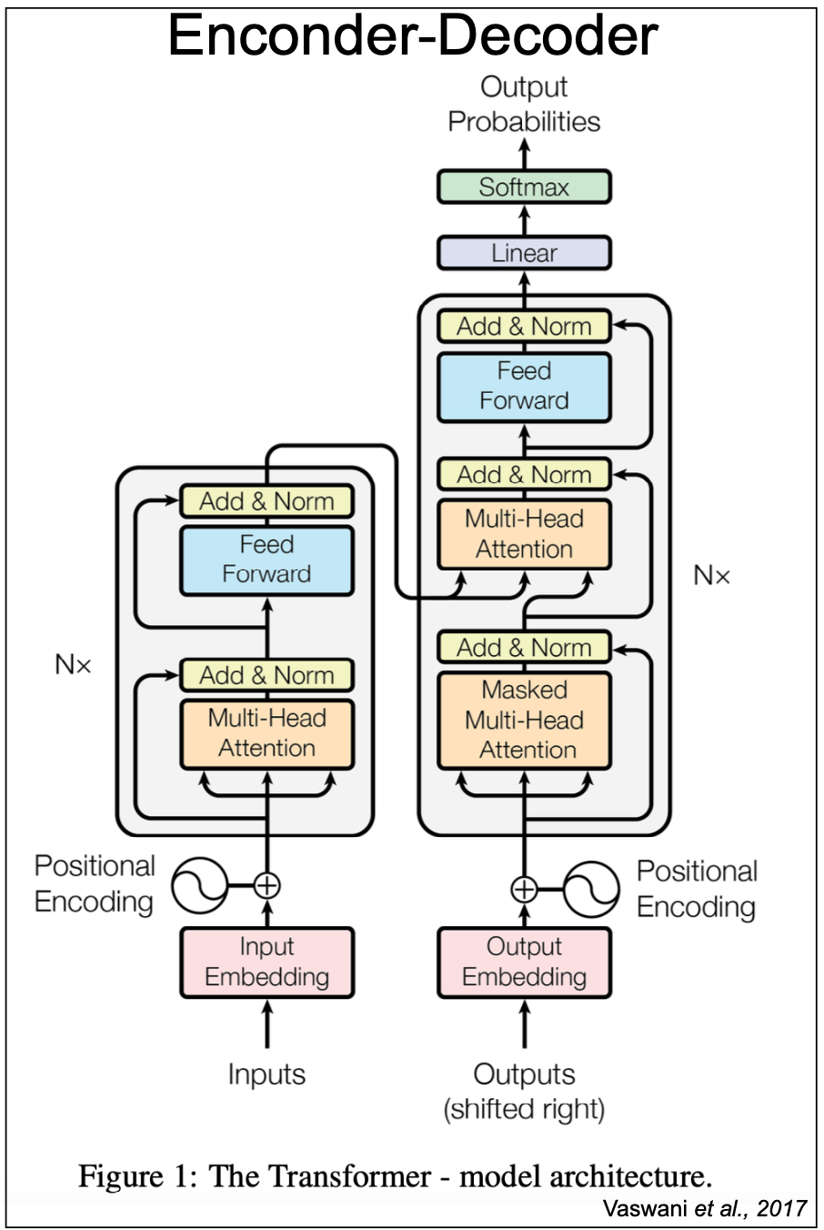
Figure 3. Vaswani et al., 2017 encoder-decoder for sequence translation.
encoder-decoder models (translation)
The 2017 Vaswani et al. paper “Attention is all you need” introduces an encoder-decoder for sequence translation using transformers. In fact, this is the manuscript that introduced the concept of a “transformer block” based on the attention mechanism. See Figure 3.
Pytorch code to implement a transformer-based encoder-decoder can be found here.
The Vaswani encoder is the same as the transformer-encoder described in Figure 2B. The Vaswani decoder has all the elements of the transformer-encoder described in Figure 2A using masked self-attention. In addition, the Vaswani decoder includes one more multi-head transformer block where the keys and values come from the output of the encoder, and the queries from the decoder. This additional layer is referred to as cross-attention.
Considering the case of a English-Spanish encoder-decoder, and the case of translating from English to Spanish the sentence “I am the boss” (Figure 4),
-
In training: (Figure 4, top)
In training, the English and Spanish pairs are both used. The encoder (the same as in Figure 2B) receives the “source” sentence in English and produces an output embedding for it.
The decoder uses the target sequence in Spanish “yo soy la jefa”, and for each word, it predict the next word. Unlike the a decoder-only where the probability of the next word depends only on the previous words, here the probability of the next word in Spanish depends on the previous words in Spanish plus all the sentence in English through the cross-attention mechanism.
In training, both encoder and decoder use cross-entropy as the loss. For the encoder, a fraction of the source English sequence is masked, and the encoder maximizes the probability of the masked residue being correct. Each masked word adds a term to the encoder cross-entropy loss.
The decoder uses autoregression and adds a loss term for each word in the Spanish target sequence, as it depends on the previous words of the target (Spanish) sequence and all the words in the source (English) sentence
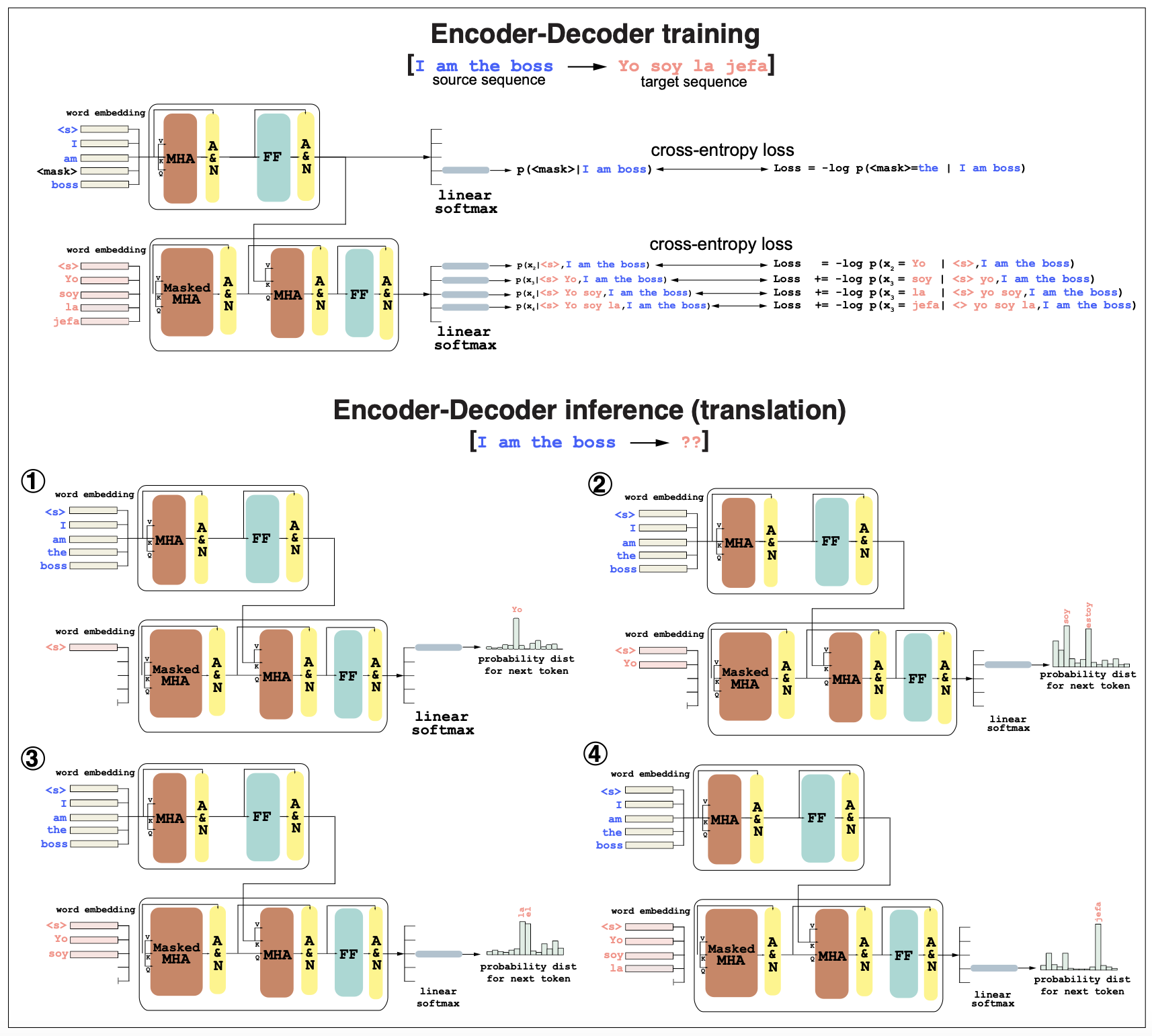
Figure 4. (Top, training) The source sequence in English "I am the boss" and the target sequence in Spanish "yo soy la jefa" are used to train an encoder-decoder for sequence-to-sequence translation. (Bottom, inference) The sequence "I am the boss" is passed to the encoder-decoder to get a translation in Spanish. MHA = multi-head attention. FF=Feed Forward network. A&N = add and normalize.
-
In translation (inference): (Figure 4 bottom) In inference mode, the input is the sequence in English “I am the boss” and the output would be its translation to Spanish.
Because the encoder-decoder is autoregressive, the words of the Spanish translation are produced one at the time.
-
First, using “I am the boss” as an input to the encoder and a \(<s>\) start character as an input to the decoder, we produce a probability distribution over words for the first word in the Spanish translation. We could sample from that distribution or take the word with the highest probability, which in this case is “Yo”.
\[P(x_1 \mid \mbox{"I am the boss"}, "<s>")\] \[\mbox{arg max}\, P(x_1 \mid \mbox{"I am the boss"}, "<s>") = Yo\] -
Next, the second translated word is produce with the same input for the encoder, but now the decoder uses as input “\(<s>\)Yo”, and the output will be a probability distribution over the second word,
\[P(x_2 \mid \mbox{"I am the boss"}, "<s>Yo")\] \[\mbox{arg max}\, P(x_2 \mid \mbox{"I am the boss"}, "<s>Yo") = soy\]In this case, the alternative word “estoy” should also have a large probability, as “am” can translate to either one of those depending on context. Adding more information to the encoder will help shaping up the probability distribution of a given word, given all the other before it.
And the process continues with the next word probability conditioned on “I am the boss” and “Yo soy”, until an \("<end>"\) token is reached. (Figure 4 bottom).
-
LLM evaluation:
Decoders: perplexity
Is it expected that the smaller the loss, the better a model is. However, losses cannot be directly compared between different methods.
Perplexity offers a way to compare the losses of two different models, provided that they use the same vocabulary (or number of tokens).
Perplexity is defined as
\[PPL(x_{1:L}) = 2^{\frac{1}{L} Loss(x_{1:L})} = 2^{-\frac{1}{L}\sum_i \log_2 P(x_i\mid x_{1:i-1})} = \left( \prod_i P(x_i\mid x_{1:i-1}) \right)^{-1/L},\]-
Perplexity ranges in values from 1 (Loss = 0) to the vocabulary size |V| why ?
-
Perplexity, by taking the average over token of the loss, is independent of length of the sequence.
-
Perplexity does not depend on the log base used.
The lower the perplexity the better. Perplexity intuitively measures the number of tokens that your are hesitating between.
Encoders: evaluate downstream tasks
The evaluation of a encoder’s performance is usually performed by evaluating the accuracy in performing any of the downstream tasks built on top of the encoder. When evaluating performance for any encoder’s downstream tasks it is important to separate the data into a training set and a validation set that have similarity to each other, otherwise, performance in the testset will not be representative of general performance in data that is not similar to the training set. This overfitting is also referred to a data leakage.
For biological sequences data leakage can occur not just because the sequences in the training set share sequence similarity with those in the test set, but also when they share other properties characteristics of the molecules, such as structure for RNAs of proteins. When fine-tuning a encoder to perform structure determination either for proteins or RNA it is important that the sequences in the training and test set are not just sequence but also structurally dissimilar. Protein sequences can be as low as 20% similar to each other in sequence but still share the same 3D fold.
LLMs in genomics
DNABERT, an encoder to model DNA in genomes
The DNABERT method, Ji et al., 2021, is a quite direct adaptation of the BERT encoder for natural languages to describe the language of DNA in genomes.
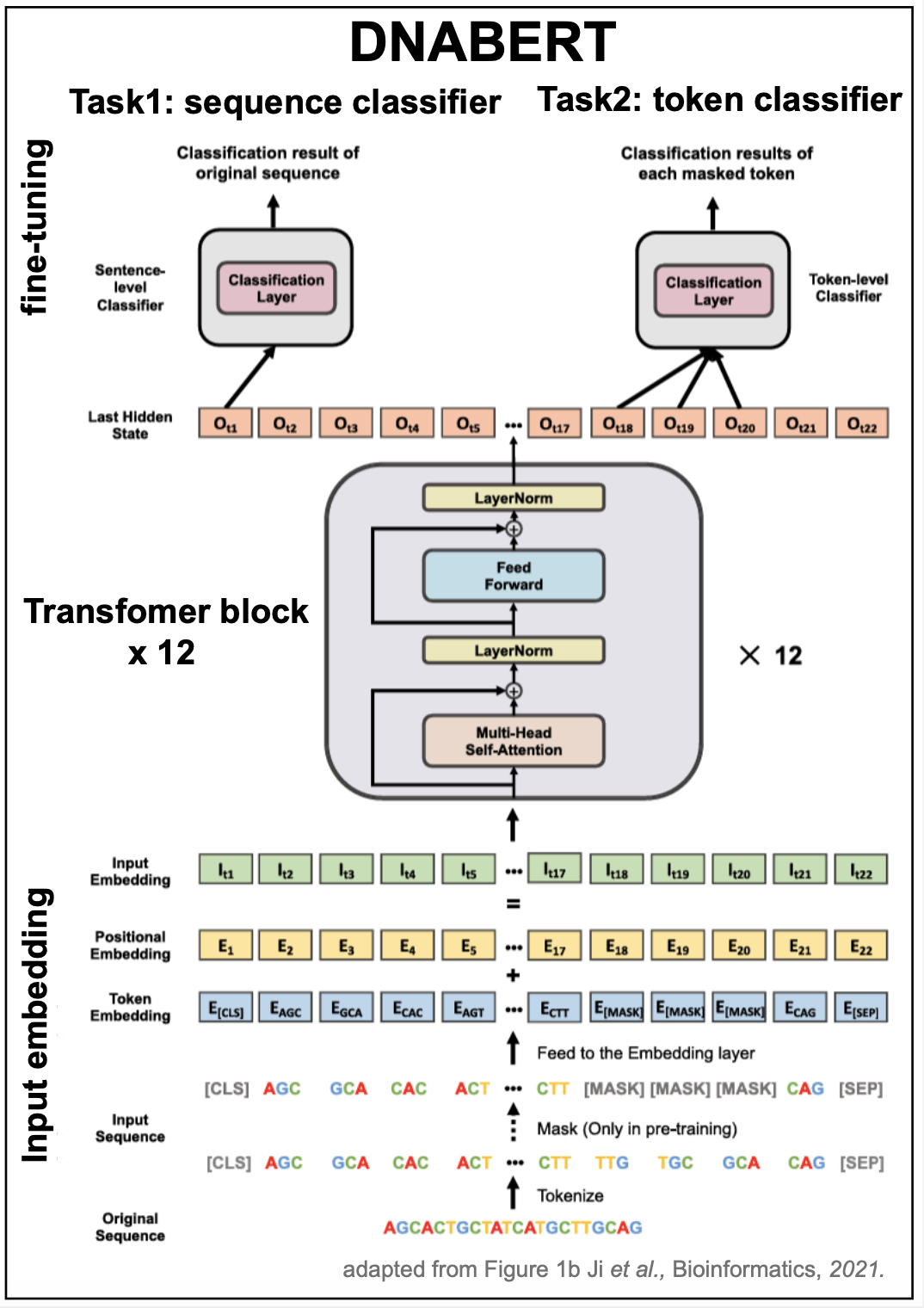
Figure 5. DANBERT model with k=3 k-mers. Adapted from Figure 1b from Ji et al. 2021.
Tokenization
Until know, we have assumed that the tokenization of a biological sequence would be by residue: nucleotide or amino acids, so that a DNA or RNA alphabet would have dimension 4, and a protein alphabet will have dimension 20. DNABERT introduces a different approach.
-
It uses k-mers (for k= 3,4, 5, or 6), so that the size of the alphabet is \(4^k\).
-
It adds five extra tokens:
-
\(>\)CLS\(>\) for classification token
-
\(>\)PAD\(>\) for padding token
-
\(>\)UNK\(>\) for unknown token
-
\(>\)SEP\(>\) for separation token
-
\(>\)MASK\(>\) for masked tokens
-
The total size of the kmer alphabet is \(4^k+5\).
Then, for a sequence “AGCTGA” according to the 3-mer alphabet includes tokens:
Pytorch code to implement a kmer tokenization alphabet can be found here
Pre-training
DNABERT pre-training is very similar to that of BERT by self-supervised training after masking \(15\%\) of the tokens on each sequence.
DNABERT uses the same model architecture than BERT (described in Figure 5). Below we give a comparison of the values of the parameters.
| model comparison | BERT | DNABERT-k | |
| vocabulary | V | 30,000 tokens | \(4^k\) + 5 |
| token size | k | k-mers: 3,4,5,6 | |
| input embedding | D | 1,024 | 768 |
| Transformer layers | K | 24 | 12 |
| Transformer heads per layer | h | 16 | 12 |
| query, key, value dimension per head | D_h | 64 | 64 |
| FF hidden dimension | d_ff | 4,096 | 3,072 |
| max length of input | Lmax | 512 tokens | 512 tokens |
| pre-training | steps | 1,000,000 | |
| pre-training | epochs | 50 | |
| pre-training | words | 3.3 billions |
Fine tuning
For each of the downstream tasks, DNABERT starts from the pre-trained parameters, and uses some task-specific data for further training (fine tuning).
Some of the tasks that DNABERT investigates are:
-
The prediction of transcription factors binding sites.
-
The prediction of proximal and core promoter regions.
-
Recognition of canonical and non-canonical splice sites.
ESM-1b (ESM-2), an encoder to model proteins
ESM-1b and ESM-2 are models that explore self-supervised language modeling applied to unlabeled amino acid sequences. They are transformer-based encoder and train in up 250 million protein sequences. Similar to DNABERT for DNA/RNA, ESM-1b and its second generation version ESM-2 they train standard transformer blocks by masked self-supervision. They are trained to predict the identity of amino acids that have been randomly masked out of protein sequences.
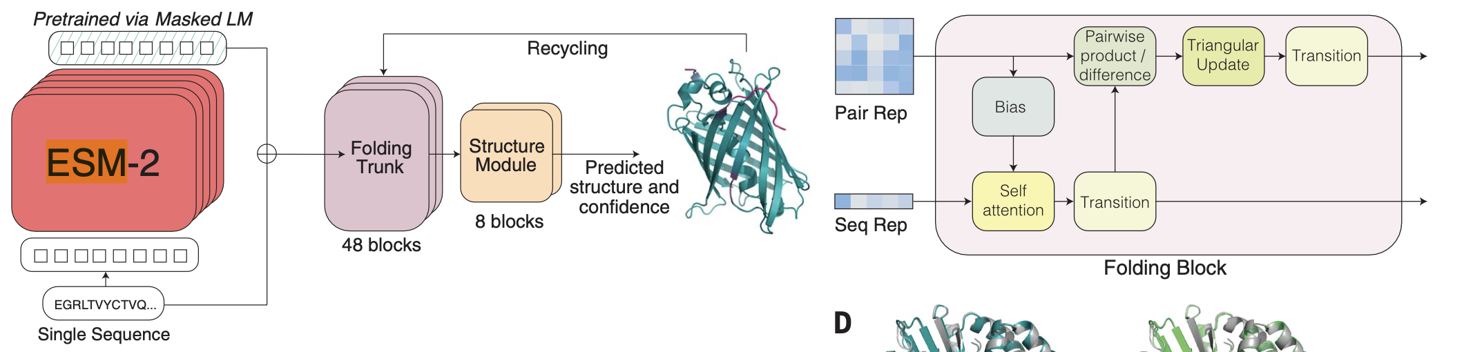
Figure 6. ESMFold architecture. Adapted from Figure 2A, from Lin et al., 2023.
fine-tuning task: protein structure prediction
ESM-2 embeddings are used as inputs to the method ESMFold described in Figure 6. ESNFold similar to AlphaFold2 predicts the 3D structure from an input protein. The input protein sequence is processed through the ESM-2 the language model, and the final ESM-2 representation is passed to the folding head.
ProGen2, an autoregressive decoder for modeling proteins
ProGen2 (Figure 7) is an example of a decoder for generating novel protein sequences.
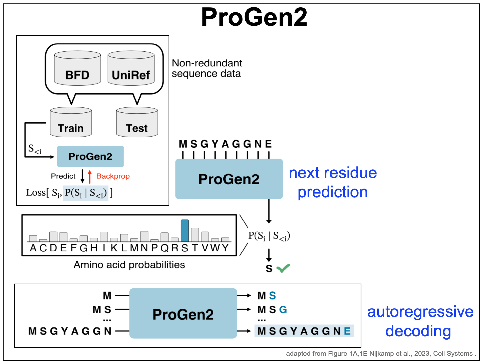
Figure 7. ProGen2 decoder for protein modeling. Adapted from Figure 1A, 1E from Nijkamp et al. 2023.
ProGen2 uses the same autoregressive decoder-only paradigm introduced by GPT3 that we have just described before (Figure 2).
-
Given an input sequence, it produces a probability distribution for the next amino acid, conditioned on the given ones.
-
The probability distribution can be use to generate the next amino acid.
-
The sequence augmented with the new amino acid, can be passed again through the model to generate the next residue.
Evo: a decoder (beyond transformers) for genomics sequences
Evo is a decoder that given a genomic sequence \(x_1\ldots x_N\), predicts the probability of the next nucleotide \(P(x_{N+1}\mid x_1\ldots x_N)\) by means of a neural network. The Evo architecture consists not just of transformers. In Evo, transformer layers are interspearsed with a different architecture named the StripedHyena architecture as depicted in Figure 8.
The difference between a transformer block and a striped hyena block resides in replacing the final FeedForward layer of a transformer by a Hyena gated block which includes convolutions, gating, and residual
Transformer block:
-
LayerNorm
-
Self-attention + residual
-
LayerNorm
-
FeedForward + residual
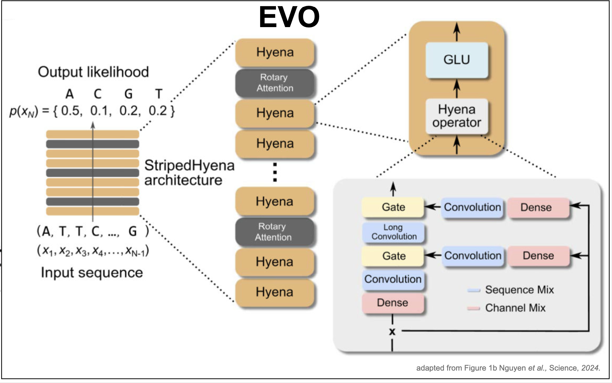
Figure 8. EVO. Adapted from Figure 1b from Nguyen et al. 2024.
Striped Hyena block:
-
LayerNorm
-
Self-attention
-
Hyena gated block, which includes:
-
LayerNorm
input x # (B, L, d_model)
residual = x
x = LayerNorm(x)
-
Two x projections: d_model = 2*hidden_dim
(B, L, d_model) -> (B, L, 2*hidden_dim)
u, v # both (B, L, hidden_dim)
-
One long convolution on u:
u_cov # back to (B, L, hidden_dim)
It is called long convolution because the filter spans most of the length of the sequence. The hope is that such long convolution will help learn long-distance interaction in sequences.
-
gating with v:
gate = torch.sigmoid(v) # (B, L, hidden_dim)
h = gate * u_conv # (B, L, hidden_dim)
-
non-linearity (RELU or GELU) and projection
h = F.gelu(h) # (B, L, hidden_dim)
h = self.out_proj(h) # (B, L, d_model)
-
residual connection
return residual + h
-

Figure 9. EVO. Adapted from Figure 1F from Nguyen et al., 2024.
Evo is trained on millions of prokariotic and phage genomes. Thus, Evo should learn foundational properties of DNA, RNA and also proteins though the information contained in the mRNA genomic sequences in the form of the tripets of nucleotides forming the codons from which the protein sequences are obtained. Evo reaches 7 billion parameters trained with a context length of up to 131,072 tokens, using single-nucleotide, byte-level tokenization.
The objective is por Evo to learn functional properties of regulatory DNA, non-coding RNAs and proteins. The paper describes several “zero-shot function prediction across DNA, RNA, and protein modalities”. What does this mean?
-
First, they evaluate perplexity. Remember that perplexity ranges from 1 to the alphabet size (4 in this case), with 1 being perfect inference with zero loss, and 4 representing a random assignment.
In Figure 1F of Evo, we observe that perplexity does not get much better than 3.1 (Figure 9). It would be interesting to compare with other ML models such as nhmmer (a hidden Markov model for genomic sequences) to see how they compare on achieved perplexity.
-
Next, they use protein and RNA deep mutational screening (DMS) data to test the Evo model using zero-shot learning. DMS data results from making mutations on the sequences and testing their effect on fitness. Zero-shot learning means that you test the accuracy of the model in predicting the fitness of the mutated sequences without having trained the model to recognize the properties to be tested.
-
One observation in the paper is that when tested “on DMS datasets of human proteins, Evo is unable to predict mutational effects on fitness (fig. S8A and table S5), most likely because the pretraining dataset is composed of prokaryotic sequences.”