MCB128: AI in Molecular Biology (Spring 2026)
(Under construction)
(Now hiring TFs Fall 2026)
- Introduction
- Autoencoder definition
- Autoencoder application: Gene expression
- Variational Autoencoders (VAE)
- The VAE decoder is a generative model
- The VAE encoder is an inference model (approximate inverse of the generative model)
- The Variational Inference approach
- Where is the deep learning part of a VAE? VAE are Deep Learning Variable Models (DLVM)
- Two optimization objectives. One method to achieve them both: The Evidence Lower Bound (ELBO)
- The reparameterization trick
- VAE Pytorch code
- Connection between Autoencoders and VAE?
- scVI: VAE for single-cell transcriptomics
- scVI architecture
- Uses: clustering.
- Uses: differential gene expression.
block 5: Autoencoders, Variational Autoencoders/Gene expression, scRNA-seq
Introduction
Autoencoders are a form of neural networks that are mostly used to extract a compressed representation of the input data. Autoencoders are trained unsupervised, that is, at training the only goal is to reproduce at the end the same values that were put in. What can we learn by this simple exercise?
The input data to an autoencoder usually has high dimensionality, and the network introduces a number of layers that progressively reduce the dimensionality (the encoder) until it reaches a lowest dimension, called the bottleneck. Once the bottleneck has been reached, the same or similar layers are applied backwards (the decoder) in order to reverse the processes. The decoder layers keep increasing the dimensionality until the input dimension is restored.
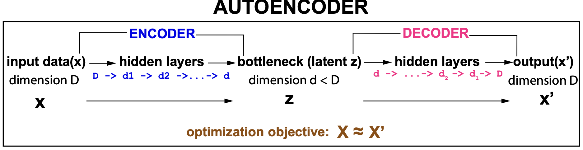
Figure 1. Schematic description of an autoencoder
In an autoencoder, the bottleneck layer can then be interpret as a low-dimensional representation (for feature extraction) of the multidimensional data.
An autoencoder is unsupervised. The leaning task is simply to achieve \(x^\prime \approx x\).
Learning as communication
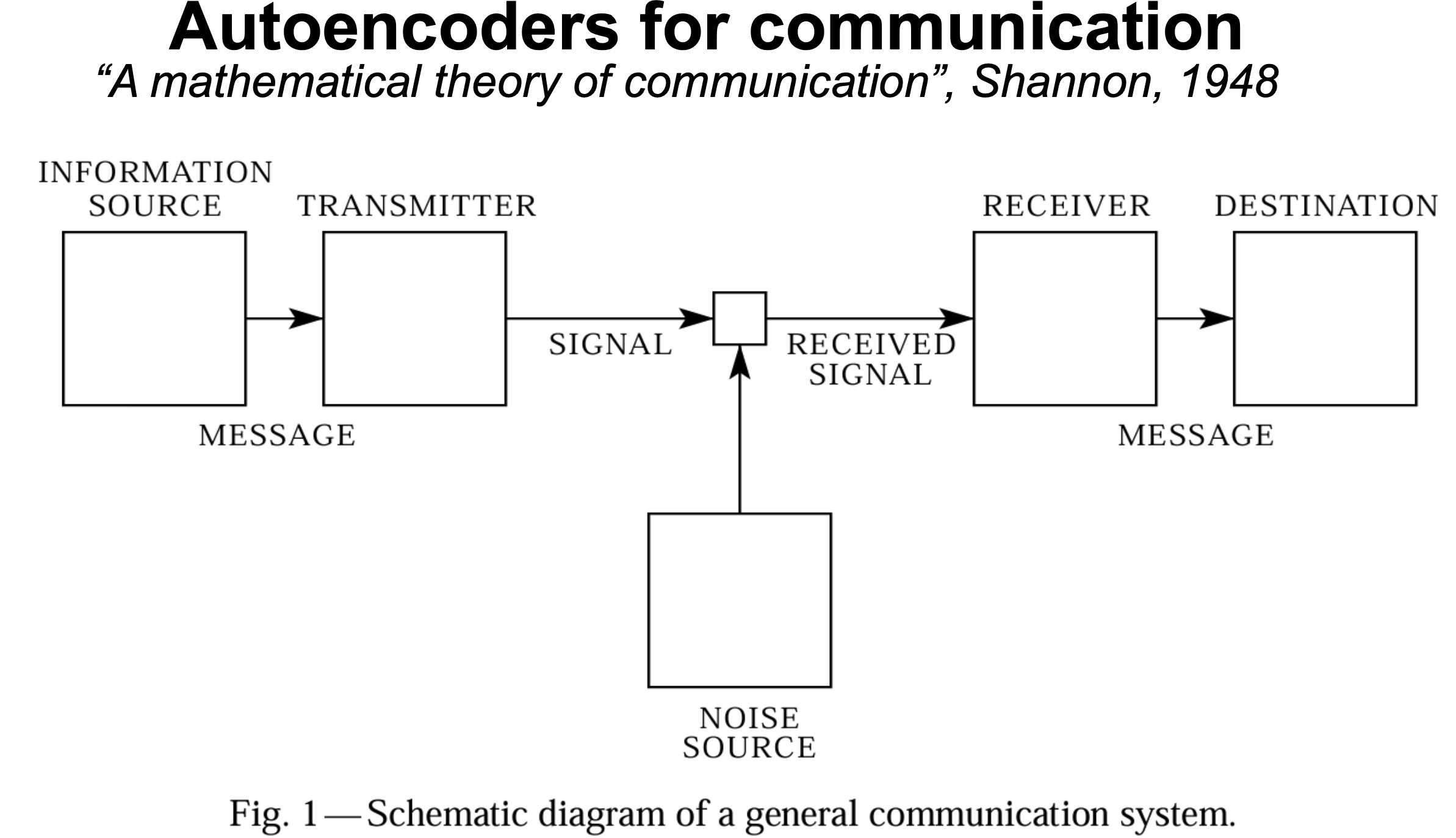
Figure 2. From Shannon's 1949 paper "A mathematical theory of communication", 1948.
Autoencoders (and learning in general) have an important connection with the field of communications. As stated in Shannon’s famous 1948 paper, any communication system depends on a source, a transmitter and a receiver (Figure 2). Shannon’s description of a communication channel in Figure 2 looks a lot like an autoencoder as described in Figure 1.
In communications, we would like to investigate what is the minimal size of the channel (the latent variable z for us) that allows a faithful transmission of the information.
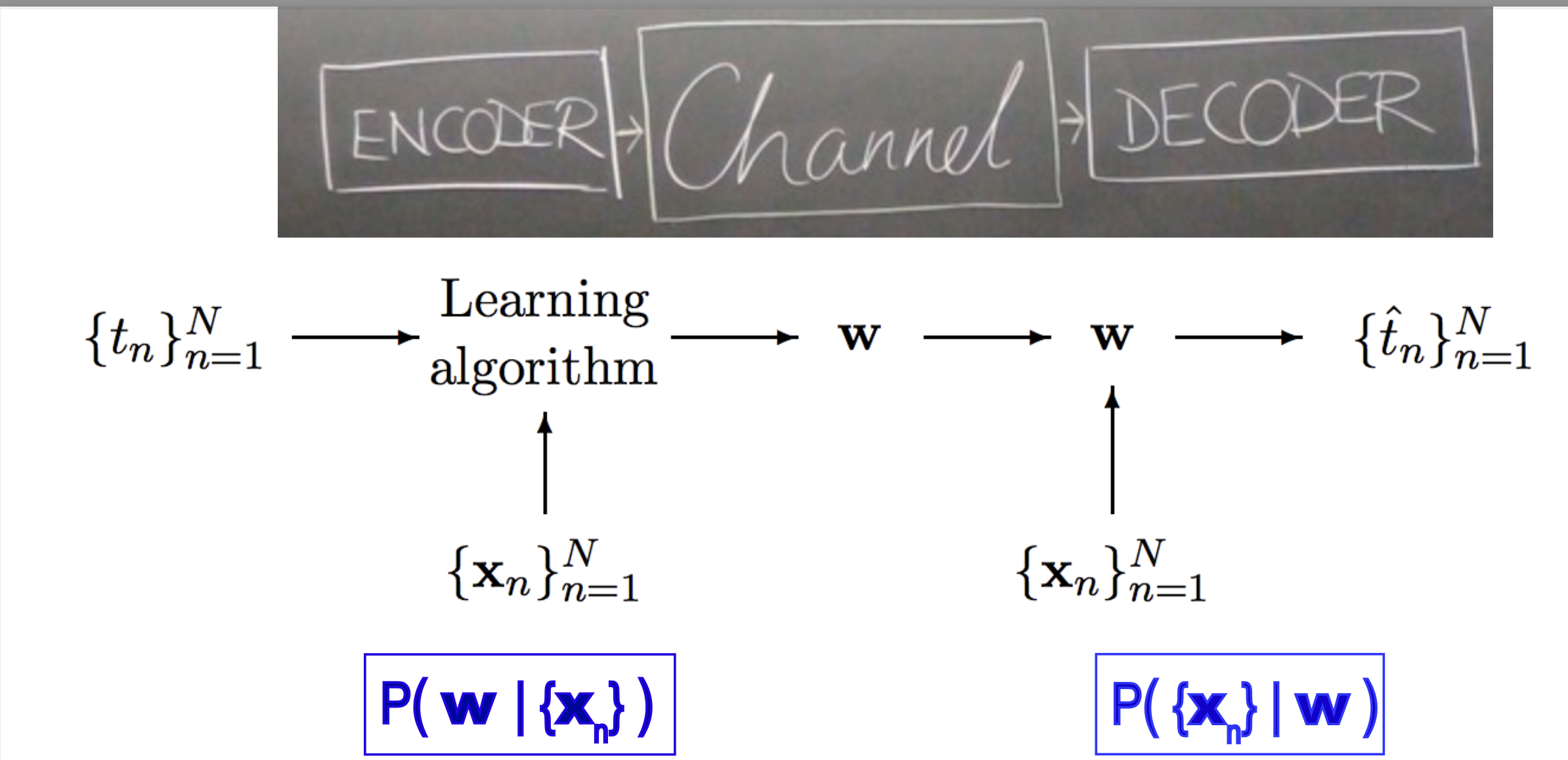
Figure 3. From MacKay's book, chapter 40 "Learning as communication".
Similarly, as described in MacKay’s book, chapter 40, and I am paraphrasing, autoencoders involve the production of a set of latent values (z) by a transmitter (or encoder) in response to an input data point (x). The decoder (or receiver) uses the latent values (z) to reconstruct the input data. Thus, the latent variable plays the role of a communication channel transporting the information contained the input data, so that it can be reconstructed faithfully and economically.
Variational Autoencoders (VAE)
In this block we are also going to discuss Variational autoencoders (VAE). VAE are a particular type of autoencoder in which we do not just try to identify a latent value z for each x, but a probability distribution \(p_\theta(z\mid x)\), that depends on some parameters here represented by \(\theta\).
A VAE decoder does not just produce one output \(x^\prime\) per input but a probability distribution \(p_\theta(x)\), the marginal probability of the data given the generative model, that we hope matches the data probability distributions \(p_{data}(x)\). And the objective is to approximate \(p_\theta(x) = \int_z p_\theta(x\mid z)\, p_\theta(z)\) to \(p_{data}(x)\)
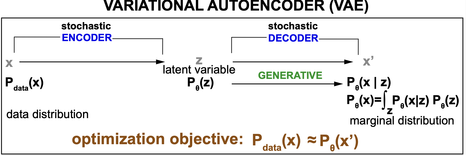
Figure 4. Schematic description of a variational autoencoder (VAE).
VAE bring us into the realm of generative models. The rest of the models we will discuss in our last block 6 will be all generative. There is a major division in the world of modeling and machine learning between discriminative and generative models. Discriminative models are defined by a conditional probability \(p(z\mid x)\) that expresses the latent variable only as a function of a given input \(x\). A generative model is defined by a joint distribution \(p_\theta(x,z)\) of all the variables (observed data x, and latent variables z). See Figure 4. A generative model is usually parameterized by two probability distributions \(p_\theta(x\mid z) p_\theta(z)\). A discriminative (inference) model can only be used to predict labels (z) for any given data point (x). A generative model, can be turn into a discriminative model, and in addition can perform unique tasks such as
-
Calculate the probability assigned to the model for any data point x, or density, \(p_\theta(x)\).
-
Sampling to generate new data points from the model distribution, \(x_{sample}\, \sim\, p_\theta(x)\).
-
Unsupervised learning, Given just data points x (but not labels), to learn the value of the parameters that maximize the marginal density \(p_\theta(x)\), and by that hopefully identify important associations in the lower-dimension latent variable(s). Here is an example extracting associations from clinical data using a VAE.
Our practical examples
As our practical case, we are going to use autoencoders to process gene expression data from many different cells. The goal is that the autoencoder will provide a lower-dimension representation of the gene expression patterns that could allow us to identify for instance cell states (cancer or otherwise) dependent on the expression (or lack there off) of distinct groups of genes.
As our practical case for a variational autoencoder (VAE) we will discuss the method single-cell variational inference (scVI) which is used for the analysis of gene expression in single cells for datasets including hundreds of thousands of cells.
documentation
Some documentation: this is a good detailed autoencoder’s reference. This is the foundational paper that introduced autoencoders, “Reducing the Dimensionality of Data with Neural Networks”, by Hinton and Salakhutdinov, 2006. The paper describes AE as a non-linear generalization of PCA (why?). This is an excellent primer on VAEs
Autoencoder definition
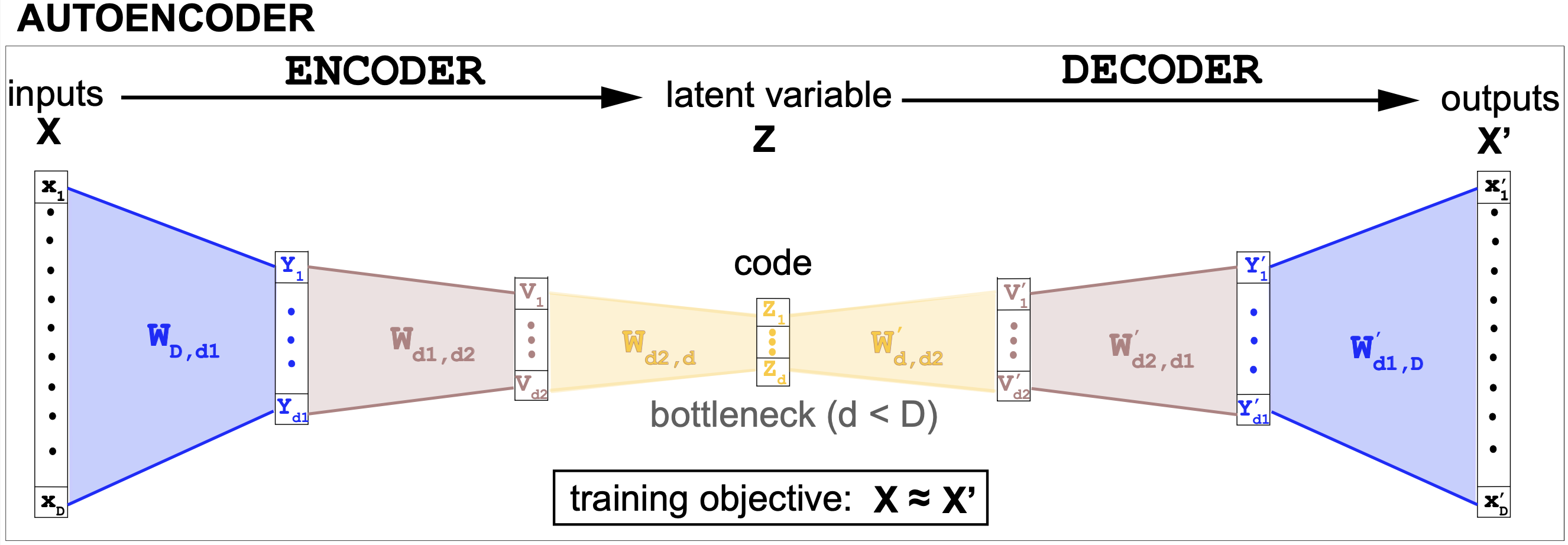
Figure 5. An autoencoder architecture. This is an example of an undercomplete symmetric encoder/decoder architecture. All the hidden layers include a non linear activation, and optionally dropout as well.
The encoder
The encoder is a sequence of fully-connected neural network layers. The encoder layers progressively reduce the dimension of the features.
For instance, in the AE code described in Figure 5, the dimensions go: from D=2000 to d1 = 512, d2 = 256, and d = 32. The last layer of the encoder outputs the latent variable (z) also referred to as “the code” or the hidden variable.
The bottleneck
The bottleneck is the core of an AE. The bottleneck is the output of the last encoder layer \(z[d]\). This latent variable is expected to learn a compact representation of the data, and hopefully provide insights about the data that cannot be seen directly from the data due to its large dimensionality.
The decoder
The decoder has an architecture that usually is the reverse of the encoder, although that is not necessary. The decoder just needs to produce an final output in the dimensions of the input data.
The activation of the last layer of the decoder is important because the output has to match the input.
-
If the input data is continuous and not bounded, a linear activation (that is, no activation) is appropriate. The output will be unbounded real values just as the inputs
-
If the input data are normalized values bounded to be between 0 and 1, then a sigmoid activation is appropriate for the last output layer. Then the output values will be normalized values bounded to be between 0 and 1, just as the inputs.
-
If the input data represent a categorical distribution of Bernoulli parameters (a one-hot encoded is a particular case of categorical distribution), then a softmax activation is appropriate.
in the code described in Figure 7, the input data is continuous and unbounded (generated as samples of a normal distribution of zero mean and variance one), thus the decoder does not use any non-linear activation for its last layer.
The AE loss
The training objective of an AE is to recover the input values. The type of data determines the loss used. For instance, for continuous input data and no activation, the loss is often the Mean Squared Error (MSE),
\[MSE(x,x^\prime) = \frac{1}{D} \sum_{i=1}^D (x_i - x_i^\prime)^2.\]If the data and reconstructions are categorical \(0\leq x_i,x^\prime_i \leq 1\) and \(\sum_{i=1}^D x_i = 1\), \(\sum_{i=1}^D x^\prime_i = 1\), one can use the cross-entropy loss
\[CrossEntropy(x,x^\prime) = - \frac{1}{D} \sum_{i=1}^D x_i \log{x^\prime_i}.\]The AE learning
In an autoencoder, the encoder and the decoder are trained together using the standard backpropagation method that we have introduced and described before. Both the encoder and decoder weights are adjusted together until reconstruction is achieved and \(x^\prime \approx x\).
As for the usefulness of the latent variable or code z, if the bottleneck dimension is insufficient for the capacity of the data, optimization will not be possible.
Undercomplete and overcomplete autoencoders
The autoencoders we have discussed so far are undercomplete, which means that the dimension of the code (or latent variable) d is smaller than that of the input data D (\(d<D\)).
There are also overcomplete autoencoder for which the dimension on the latent variable is larger than the dimension of the input data, \(d > D\). Overcomplete autoencoders seems counterintuitive, what can the AE learn by passing the input to the output without need to make any compression? It could just pass it “as is”. This is often referred to as the identity problem.
Looks like overcomplete autoencoders while not useful for extracting common features in the data, they are useful for denoising. They can learn to reconstruct an original from a noisy version of it.
Autoencoder application: Gene expression
As an example of an AE, we are going to discuss the GENEEX autoencoder introduced by the National Cancer Institute to model cancer biology data.
GENEEX is an autoencoder that takes as inputs the expression profiles of all the genes of individual cells and collapse them into latent variables of much lower dimensionality. GENEEX used the genomic expression data (RNA-seq) from cancer samples trained on 3,000 RNA-Seq gene expression profiles containing 60,484 genes from the Genomic Data Commons.
Inputs
The inputs for a gene expression autoencoder are counts of the number of RNA-seq reads associated to a given gene (g) in a given cell (c). All RNA-seq methods have their way of estimating these counts per gene (or per gene transcript), counts[c,g].
Raw counts cannot be used to compare between different samples due to
-
different libraries have different sequencing depths
-
some samples may have more RNA than other.
To avoid these confounding factor, often counts are given normalized, that is, scaled so that each cell has the same number of total counts,
\[norm\_counts[c,g] = \frac{counts[c,g]}{\sum_{g^\prime}counts[c,g^\prime]}\]and then log-transformed,
\[log1p(norm_counts[c,g]) = log(1+ norm\_counts[c,g]) \geq 0.\]Outputs
The outputs of this autoencoder are just real values resulting for the last layer of the decoder without ReLU.
GENEEX autoencoder architecture
The GENEEX autoencoder architecture includes two hidden layers of dimensions \(h_1=2,048\), \(h_2=1,024\) and latent_dim\(=128\). The encoder and decoder have a symmetric configuration. All layer except the last one of the decoder use ReLU and dropout.
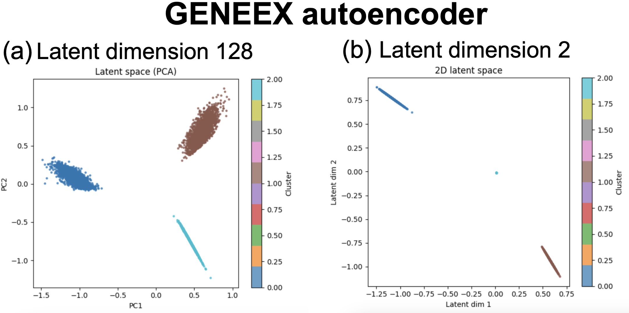
Figure 7. GENEEX AE results for synthetic data including three different gene profiles. Data include 6,000 cells each with expression data for 1,000 genes. (a) the dimension of the latent variable is 128. (b) latent variable dimension is 2.
Results
This code includes a toy example using log-transformed gene expression values for 6,000 cells each including expression data for 1,000 genes. The data has been set up such that for each third of the cells (2,000 cells), a third of the genes have high expression (up-regulated) and all the others just some background expression.
The autoencoder is easily self-trained to reconstruct the expression inputs (no labels of to which of the three classes each cell belongs to) using the MSE loss.
For an AE with latent dimension 128, we can extract the latent variables \(z[c,128]\) and using PCA, we can plot the first two PCA dimensions (Figure 7a) which clearly separate the three kind of cells. Even more simply, using a latent dimension of 2, we can directly plot the two hidden components (Figure 7b) which also allow us to infer the three different types of expression profiles present in the data.
Autoencoders as a non-linear generalization of principal component analysis (PCA)
Autoencoders are often described as non-linear generalizations of PCA.
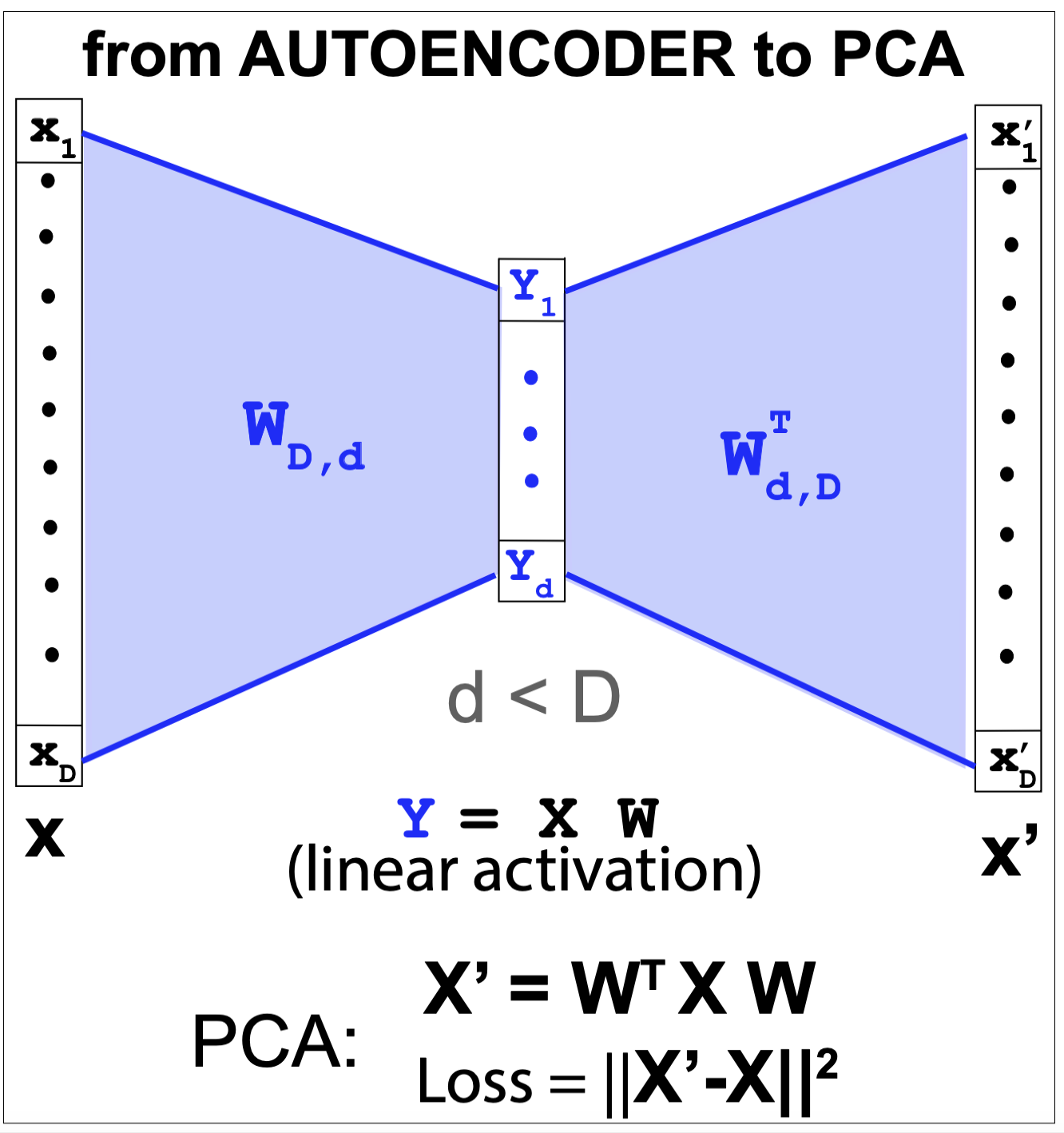
Figure 6. From autoencoder to principal component analysis.
An autoencoder is equivalent to PCA under the following simplifications (described also in Figure 6)
-
The encoder and decoder have no hidden units, only the input, output and bottleneck layer, with \(d < D\),
\[x[d]\rightarrow y[d] \rightarrow x^\prime[D]\] -
The layers are linear, no non-linear activation is added
-
The encoder and decoder share the same weights
\[\begin{aligned} y[d] &= x[D] @ W[D,d]\\ x^\prime[D] &= y[d] @ W^T[d,D] \end{aligned}\] -
Weights \(W[D,d]\) are updated using the minimum squared error (MSE) loss
\[Loss = ||x^\prime - x||^2\]
Thus, autoencoders generalize PCA by adding non-linearity in the form of hidden layer with non-linear activation functions.
Variational Autoencoders (VAE)
Here is the VAE code describing the methods for this section.
Variational autoencoders (VAE) are a particular flavor of autoencoders that use probabilistic modeling. Figure 8 provides a first summary comparing the two. An AE goal is to reconstruct all data points in the input set by means of a latent variable associate to each data point. The VAE objective is to reconstruct the data probability distribution by means of a parametric generative model. The VAE generative model introduces a probability distribution that describes both the input and the latent variables.
Thus, while the optimization objective of an AE is for each data point x that the outcome of the AE \(x^\prime\) to satisfy
AE: \(x\approx x^\prime (z)\)
by means of the bottleneck latent variable z.
The optimization objective for a VAE is
VAE: \(P_{data}(x) \approx P_\theta(x)\)
Where the marginal probability \(P_\theta(x)\) is obtained by means of the latent variable and the generative model \(P_\theta(x,z)\) as
\[P_\theta(x) = \int_z P_\theta(x,z)\, dz = \int_z P_\theta(x\mid z)\, P_\theta(z)\, dz.\]Unfortunately, it is normally intractable to obtain and to optimize this marginal distribution. That is where the “variational” part of a VAE comes into play as we will see briefly.
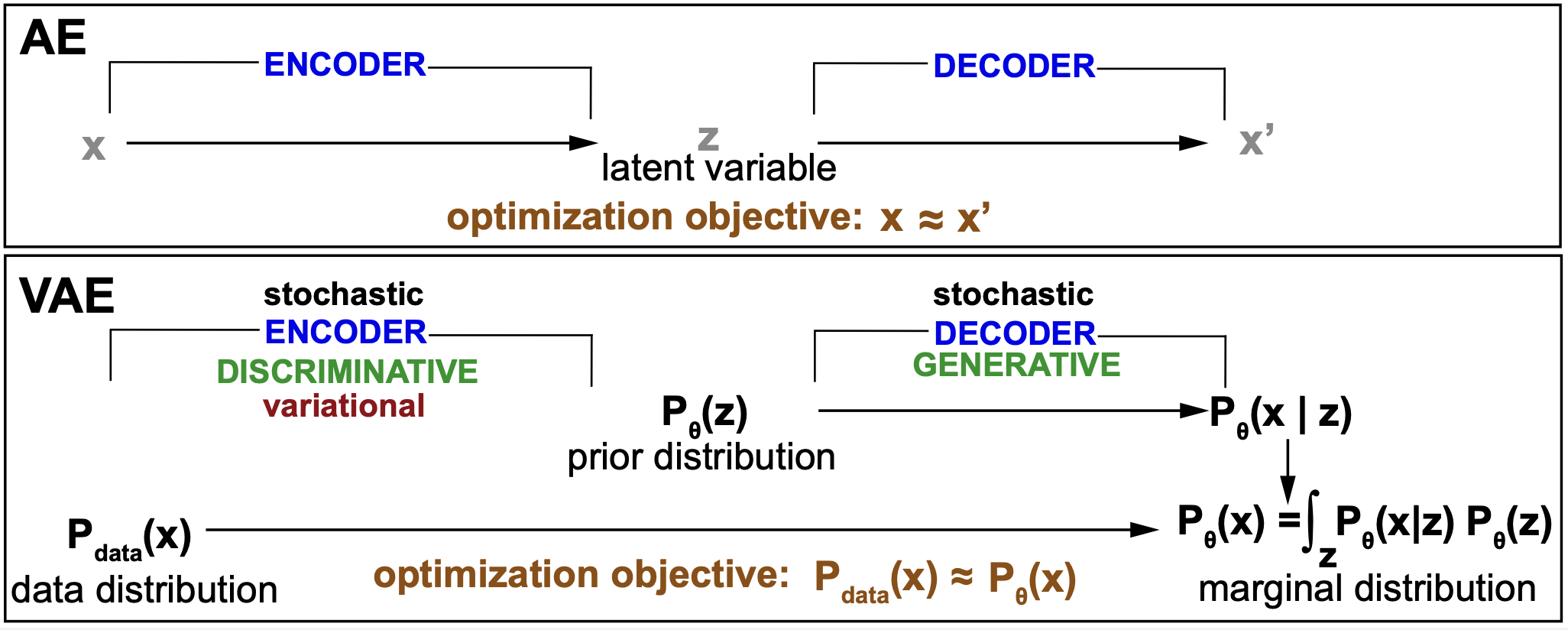
Figure 8. Summary comparison between an AE and a VAE. The "variational" component of the VAE is explained in Figure 9.
The VAE decoder is a generative model
Thus, VAE are generative models (Figure 8). That means, that they introduce probability distributions to describe all variables involved, both observed (x) and latent (z). Those probability distribution are arbitrary for each problem and depend on specific parameters that we designate as \(\theta\).
The probability distribution that describes all variables is referred to as the joint probability distribution. \(P_\theta(x,z).\)
It is common for this joint probability distribution to be factorized using Bayes theorem as
\[P_\theta(x,z) = P_\theta(x\mid z)\, P_\theta(z),\]where \(P_\theta(x\mid z)\) is the inference or discriminative distribution what gives us a probability distribution over x given a value of z, and \(P_\theta(z)\) is the prior distribution over the latent variable. See Figure 8.
Standard VAEs model these two distributions separately. The prior distribution informs about the latent variable in the absence of any knowledge about the data. It is common in VAE to model it by an Normal distribution
\[P_\theta(z) = N(0,1).\]The VAE decoder probability \(P_\theta(x\mid z)\) can be any distribution, and is usually determined by the type of data. For instance, in Figure 10, I have assumed it is a categorical distribution,
\[P_\theta(x_i\mid z) = p_i\quad for 1\leq i\leq D, \quad with \sum_{i=1}^D p_i = 1,\]thus, there is a softmax at the end of the last decoder layer. In the scVI model we are describing next, they use a negative binomial distribution.
The VAE encoder is an inference model (approximate inverse of the generative model)
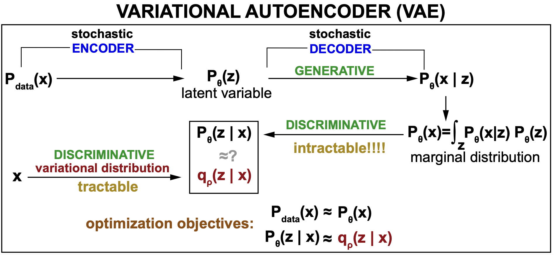
Figure 9. General description of a VAE.
The Variational Inference approach
The main idea behind variational inference (VI) is this, when you would like to find an intractable distribution, such as the posterior of a generative model \(P_\theta(z\mid x)\), then
-
Pick a different but otherwise arbitrary distribution with different parameters \(q_\varphi(z\mid x)\).
-
Use an optimization method to find the set of parameters (both \(\theta\) and \(\varphi\)) that make \(q_\phi(z\mid x)\) close to \(P_\theta(z\mid x)\).
-
Use \(q_\varphi(z\mid x)\) with the fitted parameters as a proxy for the posterior \(P_\theta(z\mid x)\) that we really want.
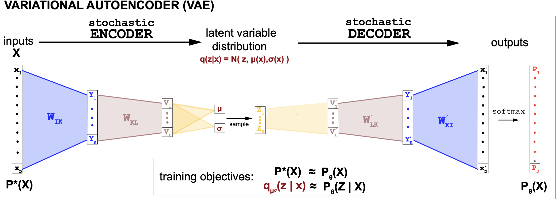
Figure 10. Description of a VAE where we assume that the generative distribution (decoder) is a categorical variable, and the variational discriminative distribution is an normal distribution where the parameters mu and log(sigma) are trained by the encoder.
Thus the VAE encoder is an inference (discriminative) model (\(q_\varphi(z\mid x)\)) that is the approximate inverse of the discriminative model (\(P_\theta(z\mid x)\)) derived from the generative model (\(P_\theta(x,z)\)), see Figure 9.
Where is the deep learning part of a VAE? VAE are Deep Learning Variable Models (DLVM)
Deep Learning Variable Models (DLVM) are generative models \(P_\theta(x,z)\) where the parameters of the model \(\theta\) are obtained by training a neural network.
A VAE uses neural networks architectures to train all the parameters involved: the encoder parameters \(\varphi\) as well as the decoder parameters \(\theta\).
Two optimization objectives. One method to achieve them both: The Evidence Lower Bound (ELBO)
The two optimizations objectives in a VAE are
-
\(P_{data}(x) \approx P_\theta(x) = \int_z P_\theta(x,z)\) (the generative model’s marginal fits the data)
-
\(q_\varphi(z\mid x) \approx P_\theta(z\mid x)\) (the inference model fits the generative model’s posterior)
A common way to measure how close two distributions are is to calculate the Kullback-Leibler (KL) divergence. The distribution that best fits the data is the one that minimizes the KL divergence
\[min_\theta D_{KL}(P_{data}||p_\theta(x)) = min_\theta \int_x P_{data}(x) \log\frac{P_{data}(x)}{P_{\theta}(x)} = max_\theta \int_{x\sim P_{data}} \log P_{\theta}(x)\]Thus, minimizing the KL divergence between the data distribution and the model’s marginal is equivalent to maximizing the log-marginal probability over the data.
For any inference model \(q_\varphi(z\mid x)\), we can write
\[\begin{aligned} \log P_{\theta}(x) &= E_{q_\varphi(z\mid x)}\left[ \log P_{\theta}(x) \right]\\ &= E_{q_\varphi(z\mid x)}\left[ \log \frac{P_{\theta}(x,z)}{P_{\theta}(z\mid x)}\right]\\ &= E_{q_\varphi(z\mid x)}\left[ \log \frac{P_{\theta}(x,z)}{q_\varphi(z\mid x)}\frac{q_\varphi(z\mid x)}{P_{\theta}(z\mid x)}\right]\\ &= E_{q_\varphi(z\mid x)}\left[ \log \frac{P_{\theta}(x,z)}{q_\varphi(z\mid x)}\right] + E_{q_\varphi(z\mid x)}\left[ \log \frac{q_\varphi(z\mid x)}{P_{\theta}(z\mid x)}\right]\\ \end{aligned}\]Because the second term is the KL divergence between the approx \(q_\varphi(z\mid x)\) and true \(P_{\theta}(z\mid x)\) inference distributions and it never negative,
\[E_{q_\varphi(z\mid x)}\left[ \log \frac{q_\varphi(z\mid x)}{P_{\theta}(z\mid x)}\right] = D_{KL}(q_\varphi(z\mid x)|| P_{\theta}(z\mid x)) \geq 0,\]then
\[\log P_{\theta}(x) \geq ELBO_{\varphi\theta}(x) = E_{q_\varphi(z\mid x)}\left[ \log \frac{P_{\theta}(x,z)}{q_\varphi(z\mid x)}\right]\]where the ELBO is the evidence lower bound
\[ELBO_{\varphi\theta}(x) = E_{q_\varphi(z\mid x)}\left[ \log P_{\theta}(x,z) - \log q_\varphi(z\mid x)\right].\]Thus the \(ELBO_{\varphi\theta}(x)\) is a lower bound to the log-probability of the data \(\log P_\theta(x)\).
And maximizing the ELBO(x) wrt both sets of parameters will result in the two things we want to do
(1) will improve the generative model by increasing the marginal \(P_{\theta}(x)\)
(2) will improve the inference model by reducing the KL distance between the true posterior \(P_\theta(z\mid x)\) and the approximate posterior \(q_\varphi(z\mid x)\).
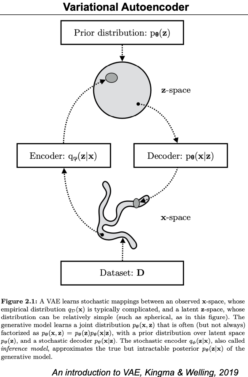
Figure 11.
The reparameterization trick
The VAE encoder (unlike a regular AE) does not produce values of the latent variable z directly, but it outputs the values of the parameters for the probability distribution \(q_\varphi(x\mid z)\).
It is typical to describe
\[q_\varphi(x\mid z) = N(z; \mu(x), \sigma^2(x)),\]thus one can sample values of z using pytorch as
\[z = torch.normal(mean, std, size=(d1,d2))\]this is an “stochastic node” not a deterministic value, and stochastic nodes cannot be differentiable, which is what we need to do stochastic gradient descend to update the parameters.
A way to avoid this problem for VAE is called the reparameterization trick.
Because z is a sample of the Normal distribution
\[z\sim N(\mu,\sigma)\quad then\quad \frac{z-\mu}{\sigma} \sim N(0,1)\]Then instead of using a non-differentiable stochastic node to sample z, we use it to sample a
\[\epsilon = torch.normal(0, 1, size=(d1,d2))\\\]and then \(z\) calculated as
\[z = \mu + \epsilon \, \sigma\]is just a deterministic value given \(\epsilon\) and can be used in backpropagation.
VAE Pytorch code
Pytorch code implementing a VAE for gene expression profiles is here
This VAE assumes that
-
The input data is log-transformed normalized counts
-
The (decoder) generative model is Normal
- Prior \(P(z) = N(0,1)\)
- \[P_\theta(x \mid z) = {N}\big(x;\ \mu_\theta(z), \sigma^2 I\big)\]
where the decoder is going to calculate \(\mu_\theta(z)\), but \(\sigma\) is fixed.
-
The (encoder) discriminative model is
\[z \sim Normal(\mu_\varphi(x), \sigma^2(x))\]were the encoder is going to optimize \(\mu_\varphi(x)\) and \(\log\sigma_\varphi^2(x)\).
-
The ELBO loss can be re-written as follows
\[\begin{aligned} ELBO_{\varphi\theta}(x) &= E_{q_\varphi(z\mid x)}\left[ \log P_{\theta}(x,z) - \log q_\varphi(z\mid x)\right]\\ &= E_{q_\phi(z\mid x)}\log \frac{ P_\theta(x, z)}{q_\varphi(z\mid x)} \\ &= E_{q_\phi(z\mid x)}\log \frac{ P_\theta(x, z)}{P_\theta(z)} \frac{P_\theta(z)}{q_\varphi(z\mid x)} \\ &= E_{q_\phi(z\mid x)}\log \frac{ P_\theta(x, z)}{P_\theta(z)} + E_{q_\phi(z\mid x)}\log \frac{ P_\theta(z)}{q_\varphi(z\mid x)}\\ &= E_{q_\phi(z\mid x)}\log P_\theta(x\mid z) - KL(q_\varphi(z\mid x) || P_\theta(z))\\ \end{aligned}\]Since the generative model is Normal, then
\[\log P_\theta(x\mid z) = \frac{-1}{2} || x - \mu_\theta(z) ||^2 + constant.\]Thus, maximizing the \(\log P_\theta(x\mid z)\) is equivalent to minimizing the mean square error
\[|| x - \mu_\theta(z) ||^2,\]Moreover, because the \(q_\varphi(z\mid x)\) and \(p_\theta(z)\) in the KL-divergence term are both Normal, there is a close form to calculate that KL-divergence term.
\[D_{KL}(N(\mu_\theta(x),\sigma^2(x) || N(0,1)) = -\frac{1}{2} \sum_{i=1}^d (1 + \log\sigma^2_i - \mu_i^2 - \sigma_i^2)\]
Connection between Autoencoders and VAE?
The autoencoder passes data through an encoder to a bottleneck layer and then it reconstructs the data from the bottleneck using a decoder. The AE bottleneck layer (Figure 1) is similar to the VAE latent variable (Figure 4). But the objectives are different
-
The VAE creates a probability distribution of the latent variable \(z\) given the data \(p(z\mid x)\).
-
The AE simply creates a low-dimensional representation of the data (one z for each x, not a probability distribution \(p(z\mid z)\)) that captures the essence of the data.
As a result,
-
The VAE creates a marginal distribution from that data from which new examples can be samples.
-
The AE only produces one \(x^\prime\) for each input \(x\).
scVI: VAE for single-cell transcriptomics
single-cell variational inference (scVI) is a variational autoencoder method for analyzing single-cell RNA-seq data. Both the scVI paper and its scVI supplement are worth reading.
Single-cell transcriptomics is the study of gene expression levels in individual cells. scRNA-seq is an extensively used high throughput technique that provides information about the expression levels of all genes in one single cell. scRNA-seq can provide information for millions of single cells in one experiment, and for each cell, it provides information about the transcriptional state of each gene.
The main information provided by an scRNA-seq experiment are the number of RNA molecules (observed counts) found associated to a given gene (g) in a given cell (n), that we represent by \(x(n,g)\).
With this information, one can do many downstream analyses such as
-
(1) To cluster cells with similar expression profiles and in that way to identify distinct cell types.
-
(2) To analyze how a type of cell present differential gene expression under two different conditions such as health/disease or any other differential conditions the cells may have been subjected to.
The scVI method encodes the transcriptome of each cell (n), \([x(n,g=1),\ldots, x(n,g=G)]\) through several fully-connected layers to a low-dimensional latent representation \([z(n,d=1),\ldots, z(n,d=D)]\), with \(D<G\). This latent representation is then decoded by another set of non-linear transformations to generate an estimate of the parameters of the probability distributions that determines the number of transcripts for each gene in each cell.
There are two important noise variables in scRNA-seq, one is the library size, the other is the batch effect. The library size refer to the fact that the
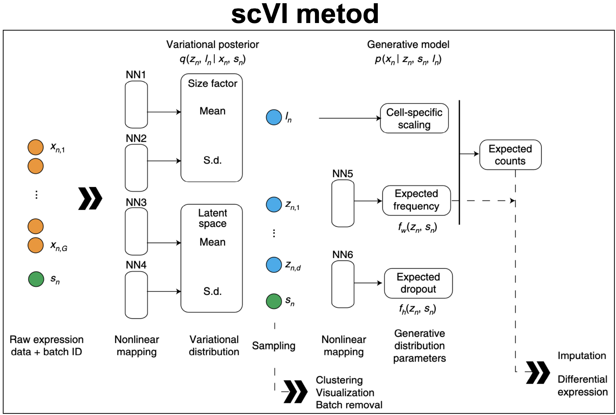
Figure 12. scVI variational autoencoder. "Deep generative modeling for single-cell transcriptomics", Lopez et al., 2018.
scVI architecture
-
The input data are the counts of the number of transcripts associated to each gene (\(1\leq g\leq G\)) in a cell (n),
\(x[n,g]\) = number of transcripts associated to gene g in cell n (see Figure 13).
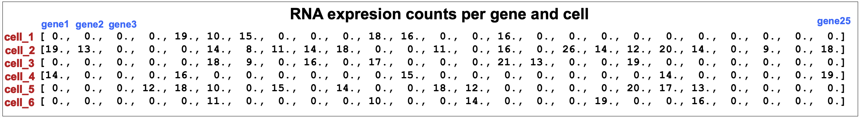
Figure 13. scVI inputs are the number of RNA transcripts associated to each gene in each cell.
-
The latent variable has dimension \(D\) for each cell n, \(z[n,d]\) for \(1\leq d\leq D\).
\(z[n,d]\) = latent variable
-
There is another latent variable, only one per cell \(l[n]\). This latent variable represent some overall scaling factor for the cell. It can be interpreted as the library size.
-
The encoder variational distributions for the latent variable \(q(z\mid x)\), are described as normal distributions, one for each gene in each cell.
-
The encoder neural network trains the parameters of the variational distribution \(\mu_x[n,D]\) and \(\log \sigma^2_x[n,D]\).
-
The decoder generative model assumes a normal distribution for the prior of the latent variable \(P(z)\)
- The decoder generative model assumes a negative binomial (NB) distribution to predict the RNA counts (c) for a given gene (g) given the latent variable.
-
The decoder trains a FC neural network to map the latent variable \(z\) to the parameters of the NB distribution \(\mu\). The \(\theta\) parameters is also trained jointly but it is not made dependent on the latent variable.
- The NB parameters \(\mu[n,g]\) are trained using the decoder FC network from the latent variables \(z\).
Actually, the decoder layers train the variables \(\rho[n,g]\) which are the expression probabilities of each gene in each cell. Then, the actual means of the NB distributions are given by
\[\mu[n,g] = l[n]\, \times \rho[n,g].\]- The NB parameter \(\theta[n,g]\) are trained without dependence from the latent variables \(z\).
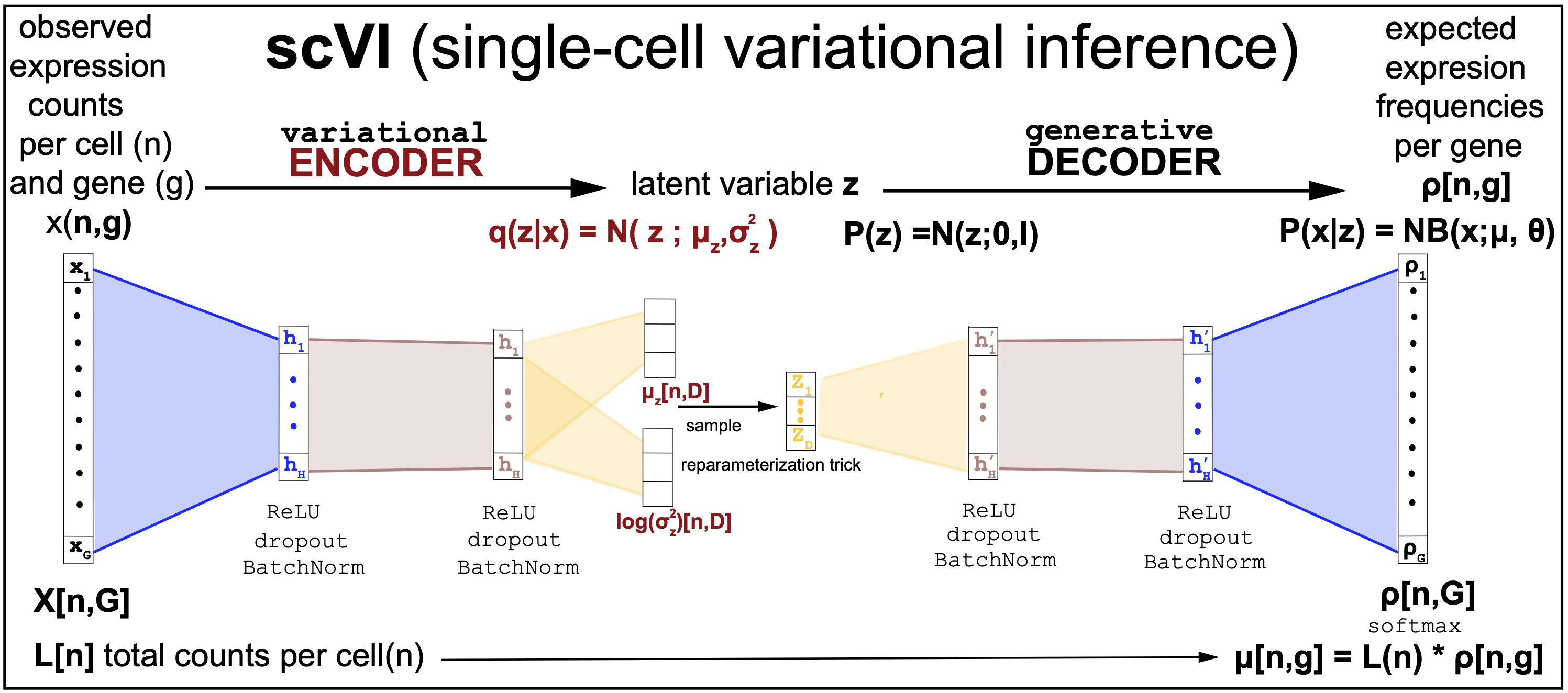
Figure 14. slightly simplified description of the scVI variational autoencoder.
- The loss is the -ELBO:
Figure 12 is taken directly from the scVI manuscript as a description of the model. Figure 13 is an simplified version of the scVI algorithm, with the corresponding scVI-simplified code.
The simplifications introduced in Figure 14 and the scVI-simplified code are the following,
-
The scVI-simplified does not train the \(l[n]\) variables, they are directly taken as the total counts of the input counts
\[l[n] = \sum_{g=1}^G x[n,g]\]Our simplification removes the need for networks NN1 and NN2 in Figure 12, used to train the mean and variance of \(l[n]\).
-
The actual distribution assumed for the counts given the latent variable in the scVI method is a Zero-inflated Negative Binomial (ZINB)
\[P(c\mid z) = ZINB(c\mid \mu(z), \theta) = \pi \delta(c=0) + (1-\pi)\, NB(c\mid \mu(z), \theta)\]The ZINB allows to describe the presence of genes with no transcripts as a result of two different causes, such as true biological absence of transcripts, and also technical dropouts.
As we see in Figure 15, everything else being equal, a ZINB allows to have many more genes per cell with zero counts, and other wit many counts.
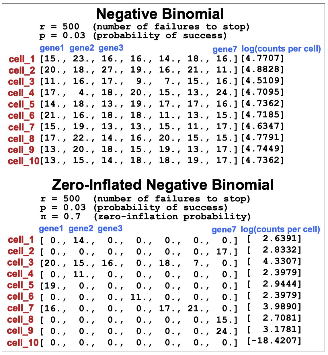
Figure 15. Comparison of counts data obtained with a negative binomial (NB) versus a zero-inflated negative binomial (ZINB).
Our simplification removes the need for network NN6 in Figure 12 used to train \(\pi[n,g]\)
Uses: clustering.
The latent variables can be used to identify cluster of cells in the latent space that could represent biological similarities amongst them. See Figure 2 in the scVI manuscript, and supplemental figures.
Uses: differential gene expression.
Using the trained variational distributions representing the data, we can make inferences about the cells. For differential gene expression analysis, given two cells, one can sample from their variational distributions in order to test the alternative hypothesis of a given gene having differential expression in those cells.
Consider two cells \(n_a\) and \(n_b\), for a given gene g, we can consider two alternative hypotheses
-
the expression of g is larger in \(n_a\) than \(n_b\),
\[H_1 = \rho(n_a,g) > \rho(n_b, g)\]where \(\rho(n_a,g)\) are the expected frequencies of expression for the gene g in cell \(a\).
-
the expression of g is smaller in \(n_a\) than \(n_b\),
\[H_2 = \rho(n_a,g) \leq \rho(n_b, g)\]
We can test those hypotheses as follows
-
Given the counts \(x_a^g = x(n_a, g)\) and \(x_b^g=x(n_b, g)\), sample latent variables from the variational distribution
\[q(z\mid x_a^g) \longrightarrow (z_a^g)^{(s_a)}\quad \mbox{Sa samples}\] \[q(z\mid x_b^g) \longrightarrow (z_b^g)^{(s_b)}\quad \mbox{Sb samples}\] -
With those sampled latent variables, using the decoder, calculate normalized expressions for the gene
- Then the ratio of the two hypotheses can be calculated as
where \(C^{(s_as_b)}(\rho_a^g > \rho_b^g) = 1\) if \((\rho_a^g)^{(s_a)} > (\rho_b^g)^{(s_b)}\) or zero otherwise; and \(C^{(s_a s_b)}(\rho_a^g \leq \rho_b^g) = 1\) if \((\rho_a^g)^{(s_a)} \leq (\rho_b^g)^{(s_b)}\) or zero otherwise.
See Figure 3 in the scVI manuscript, and supplemental figures.