MCB128: AI in Molecular Biology (Spring 2026)
(Under construction)
(Now hiring TFs Fall 2026)
- Transformers
- Transformers for multiple sequence alignments (MSAs)
- AlphaFold2: accurate protein folding with transformers
block 3: Transformers / Protein Folding-AlphaFold2
Transformers are the dominant architecture for natural language processing. Chatbots are all based on transformers. In molecular biology, transformers are behind methods such as AlphaFold2, a method to predict the 3D fold of proteins from sequences and alignments. AlphaFold was a great breakthrough in 2020 when it significantly outperformed most other methods in the CASP14 blind competition to predict recently solved protein structures.
The key component of transformers is the use of self-attention, a method to capture long-range interactions. Attention became well-known with the famous 2017 Vaswani et al. paper “Attention is all you need”. The Vaswani et al. paper describes a relatively complicated transformer, and for that reason, we will discuss it in block 4 when we study Language models.
In this block, we are concentrating on first introducing attention and how attention is used in transformers; and then we will discuss the AlphaFold2 method for protein structure prediction using transformers.
Python code for the attention and transformer mechanisms discussed in this block is here.
Transformers
Important properties of transformers that makes them preferable over RNNs are
-
Transformers naturally deal with sequences (natural language or biological) of variable lengths. With CNNs and RNNs the examples all have to have the same input dimensions. Images are easily resizeable by scaling, that is not possible for natural language sequencer or biological sequences. One cannot scale a protein sequence.
-
Sentences can be ambiguous, transformers allow every position to pay attention to their context. Attention is a mechanism that allows to learn interactions intro different part of an input. Both natural sequences and biological sequences convey important context information. For biological sequences, both RNA and protein structure leaves a signature of covariation between interacting residues. As we saw in block 0, the ribosomal binding sites depend amongst other adjacent signals on the presence of a nearby AUG start site and a TATA box sequence.
-
Self-attention allows to share parameters to deal with long inputs. The same set of attention parameters are shared for different input positions. The number of parameters become completely independent of the input length, which gives transformers a lot of flexibility as to the different sequences that one given transformer can be applied to. This is similar to how CNNs also share convolution kernels.
Self-attention
Self-attention is the mechanism behind transformers that gives them the three properties described above by means of (1) using shared parameters that do not depend of the inputs dimensions, and (2) producing parallel representations of the inputs that interact with each other to extract interaction properties contained in the sequences themselves.
Inputs
The inputs to an attention block is a sequence \(X\) of dimensions \([L,D]\), where L is the length of the sequence and each elements \(x_i\) is a \(D\) dimensional embedding vector. In natural language processing, the first step is to make the input units or tokens. For biological sequences, tokenization into residues (nucleotides or amino acids depending on the type of sequence) is trivial.
Our transformers for biological sequences take not just sequences but also alignments as inputs. The same attention weights can be used when the input is a sequence of length \(L1\) \(X[L1,D]\), or an alignment of length \(L2\) with \(S\) sequences \(X[S,L2,D]\). Only the embedding dimension has to be the same for them to be processed by the same attention weights. In Figures 1 and 2, we describe in detail the attention mechanisms in parallel with a single sequence and an alignment both with the same embedding dimension \(D\).
Queries, Keys and Values
In Figure 1, we describe the how to build the attention weights or maps. The self-attention mechanism introduces three linear transformations of the input data into queries, keys and values.
For an input \(X[L,D]\), it uses weights \(W^Q[D,d_k]\), \(W^K[D,d_k]\), and \(W^V[D,d_v]\), and biases \(b^Q[d_k]\), \(b^K[d_k]\), and \(b^V[d_v]\), to introduce the three linear transformations
- Queries \(q[L,d_k]\), such that for each sequence positions \(1\leq i\leq L\)
- Keys \(k[L,d_k]\)
- Values \(v[L,d_v]\)
The dimensions \(d_k\) and \(d_v\) are arbitrary, but in many cases they are taken as equal to the embedding dimension \(d_k=d_v=D\).
These three linear projections of the input data serve different purposes in self-attention. The “queries” and “keys” talk to each other (in a non-linear way) to produce the attention maps. The “values” carry over the result of queries and keys talking to each other to produce an output.
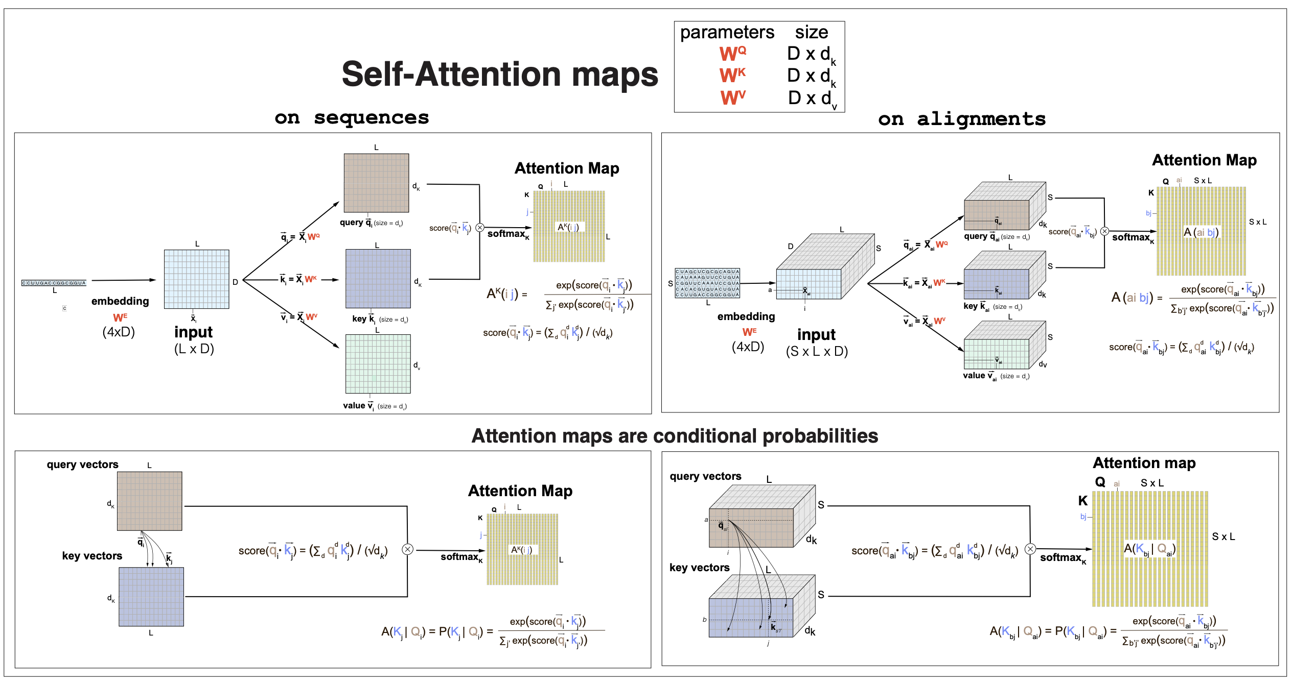
Figure 1. Self-attention maps obtained by queries and keys dot-product followed by softmax. The same attention weights can be applied to a sequence (left) or an alignment (right). The length L of the sequence (or alignment), and the number of sequences S can have any values.
dot-product self-attention maps
The attention maps \(A[L,L]\) are the result of a dot-product between queries and keys (thus, they have to have the same dimension), which is then passed through a non-linear step by using a softmax function.
A linear dot-product score between queries and keys is constructed as, for \(1\leq i, j, \leq L\),
\[\mbox{score}(q_i\dot k_j) = \sum_{d=1}^{d_K} q_i(d)\,k_j(d) \,/\, \sqrt(d_K).\]Attention dot-product scores are usually scaled by \(\sqrt(d_K)\) to avoid being dominated by the largest values.
Then the attention between positions \(i, j\) through the queries/keys dot-product score is a softmax with respect to Keys
\[A_{i,j} = \frac{e^{\mbox{score}(q_i\dot k_j)}}{ \sum_{l=1}^L e^{\mbox{score}(q_i\dot k_l)}}.\]The attention-map non linearity appears as all the keys have to compete for the attention of one query. More technically, the attention maps are conditional probabilities of all keys, given one query, such that, for each \(1\leq i,j\leq L\),
\[A_{i,j} = P(k_j | q_i) \quad \mbox{and}\quad \sum_{j=1}^L A_{i,j} = \sum_{j=1}^L P(k_j \mid q_i) = 1\quad \mbox{for each}\, 1\leq i\leq L.\]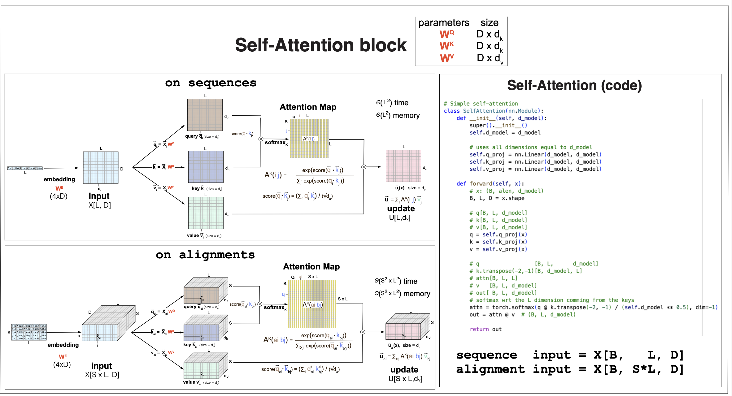
Figure 2. The self-attention block
The self-attention block
Finally, after calculating the self-attention maps \(A[L,L]\), the value vector carry over those attention interactions to the self-attention output, or update \(u[L,d_v]\), as
\[u_i[d_v] = \sum_{j=1}^L A_{i,j}\, v_j[d_v] \mbox{for}\quad 1\leq i\leq L.\]It is common in transformers to use self-attention that assigns \(d_v = D\).
In summary, a self-attention block convert an inputs of the form \(X[L,D]\) (for any arbitrary value of L) into an output or update \(u[L,d_v]\), after using a dot product that can infer context dependencies between positions, for any input with any arbitrary length L. (Or any alignment of any arbitrary length L and any arbitrary number of sequences S). See Figure 2 for a full description of a self-attention block.
Pytorch code to implement a simple self-attention block can be found here. Figure 2 shows a SelfAttention class with \(d_v=d_k=D\), for an arbitrary embedding dimension \(D\).
Matrix form
The self attention computations can be written in a compact matrix form. See Figure 3. Sometimes, it is good to see the same thing from different angles.
The notation is as follows:
-
X[B,L,D] represents a matrix with three dimensions of values B, L and D respectively.
-
An element of \(X[B,L,D]\) is described as
-
In a matrix product, we look at the last two dimensions of the two tensor, the last dimension of the first tensor has to be the same as the next-to-last dimension of the second tensor, and that is the common dimension that is multiplied and summed over.
For instance we represent,
\[X[L,D] * W[D,M] = Y[L,M]\quad \mbox{which means that}\quad y_{lm} = \sum_{d=1}^D x_{ld} w_{dm} \quad\mbox{for}\quad 1\leq l\leq L, 1\leq m\leq M.\]or more generally,
\[X[B,L,D] * W[B,D,M] = Y[B,L,M]\quad \mbox{which means that}\quad y_{blm} = \sum_{d=1}^D x_{bld} w_{bdm} \quad\mbox{for}\quad 1\leq b\leq B , 1\leq l\leq L, 1\leq m\leq M.\]The last two dimension are called the “matrix dimensions” and the other dimensions are called the “batch dimensions”.
In Pytorch, we can use torch.matmul
Y = torch.matmul(X, W)
Pytorch also has torch.einsum that allows one to do all those matrix operations in Einstein notation, in which one can specify which indices disappear. The product multiplication above is equivalent to
Y = torch.einsum('bij,bjk->bik', X, W) -
A transposition simply changes the order of the desired dimensions. For \(K[L,d_k]\) then \(K^T[d_k,L]\).
in einsum notation
K_T = torch.einsum(‘ij->ji’, K)
A note on broadcasting
What if the matrices you want to multiply do not have the same batch dimensions?
For instance, you want to multiply the last to dimensions of tensors \(X[B,L,D]\) and \(W[A,D,M]\). If you try
Y = torch.mathmult(X, W)
that will fail if \(A\neq B\) (and even if A=B but those two dimensions represent two different inputs, the result would be incorrect).
What you have to do is broadcast those dimensions. We want to trivially convert our tensors to adding the missing dimension from the other tensor (valued to one) \(X[B,1,L,D]\) and \(W[1,A,D,M]\), then this works,
\[Y[B,A,L,M] = X[B,1,L,D] * W[1,A,D,M] = torch.mathmult(X,W).\]which is a matrix representation of the operations to calculate each of the elements \(y\in Y[B,A,L,M]\) as
\[y_{balm} = \sum_{d=1}^D x_{bld} w_{adm}.\]Matrices are broadcastable in a given dimension when both tensors have the same dimension value, or one of them is 1.
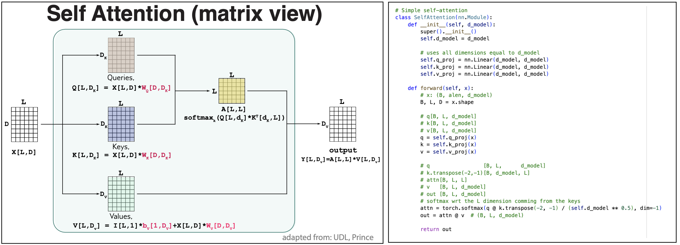
Figure 3. Matrix format to describe self-attention.
Using matrix notation as in Figure 3, we can write all operations in a self-attention block as
-
Queries, Keys and Values
\[q[L,d_k] = I[L,1] * b^Q[1,d_k] + X[L,D] * W^Q[D,d_k]\\ k[L,d_k] = I[L,1] * b^K[1,d_k] + X[L,D] * W^K[D,d_k]\\ v[L,d_v] = I[L,1] * b^V[1,d_v] + X[L,D] * W^V[D,d_v]\\\] -
Self-attention map
\[A[L,L] = \mbox{softmax}_k \left(\frac{q[L,d_k] * k^T[d_k,L]}{\sqrt(d_k)}\right)\] -
Output
\[y[L,d_v] = A[L,L] * v[L,d_v]\]
Complexity of self-attention
The time complexity of the self-attention mechanism increases quadratically with the sequence length (or quadratic with \(S*L\) for an alignment of S sequences).
The size of the self-attention maps is also quadratic on the length of the sequence.
The quadratic scaling with the sequence length both for the time to compute and the space needed to store the attention maps are taxing when we start considering many large sequences, which is usually necessary for training the parameters. Many different options have been considered to mitigate these computational and storage demands of self-attention. In the next sections we will discuss one of such approximation when we calculate attention by rows or by columns to implement alignment self attention.
Multiple-head attention
It is now easy to apply multiple attention mechanisms in parallel, that is referred to as multi-head attention.
As described in Figure 4 for the simple case of 2 heads, in general for H heads, H different sets of queries, keys, values are computed, (\(1\leq h\leq H\))
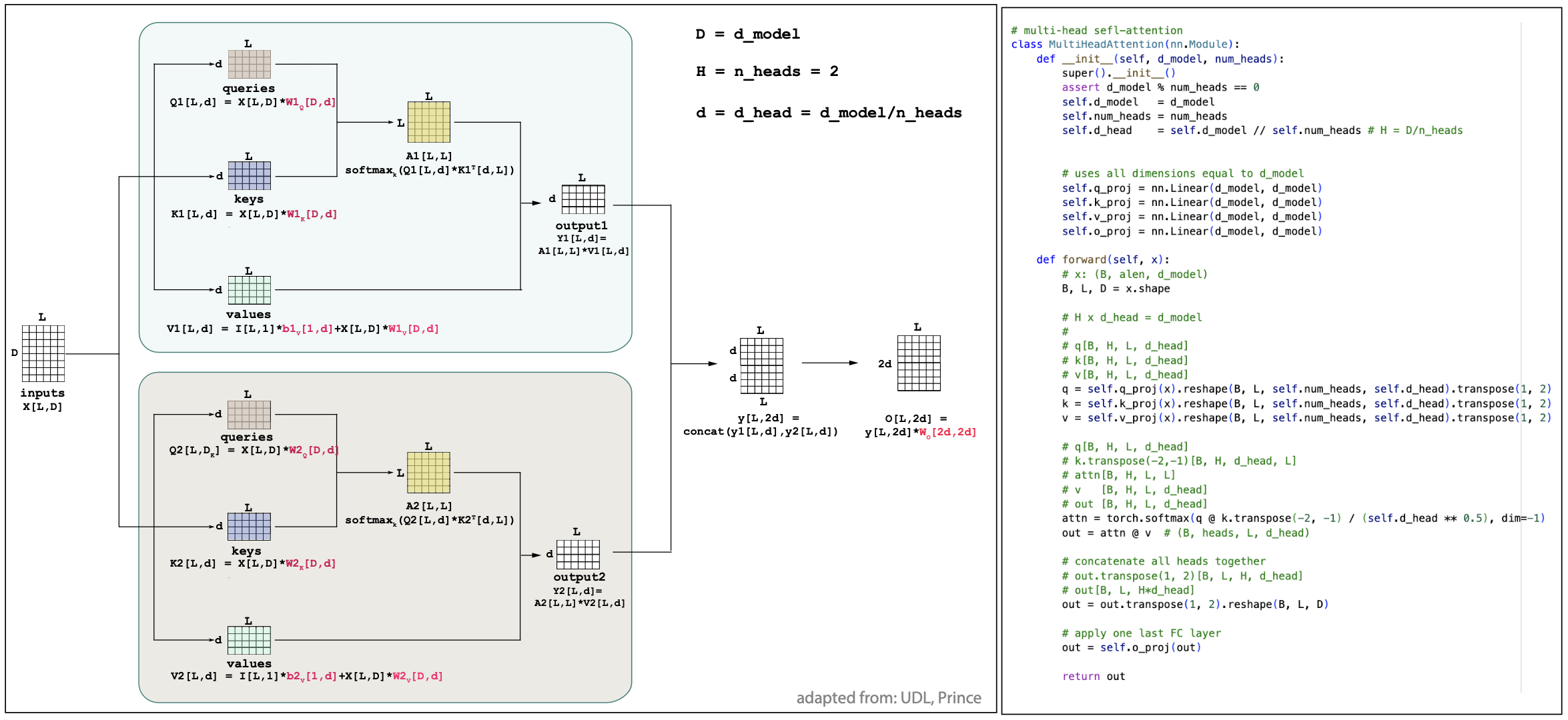
Figure 4.
which requires a set of weights \(W_h^Q, W_h^Q, W_h^Q\) and \(b_h^Q, b_h^Q, b_h^Q\) per head \(h\).
The attention maps and outputs are also calculated in parallel per head as
\[A_h[L,L] = \mbox{softmax}_k \left(\frac{q_h[L,d_k] * k_h^T[d_k,L]}{\sqrt(d_k)}\right)\\\]as well as the outputs per head
\[Y_h[L, d_v] = A_h[L,L] * v_h[L,d_v].\]Typically, if \(D\) is the inputs embedding dimension, it is typical to set \(d_k = d_v = D/H\), so that the final output embedding after concatenation is still D. In the end, as described in Figure 4, after all outputs of the individual heads have been concatenated, a final fully connected layer with weights \(W_c[D,D]\) is applied.
\[Y[L,D] = (Y_1[L,D/H],\ldots,Y_H[L,D/H]) * W_C[D,D]\]In practice, all attention mechanisms seem to be applied in a multi-head format.
Figure 5. A transformer layer. Inputs are X[L,D] D-dimensional embedding of the L input residues. The outputs have the dimensions {L,d_v]. It is standard, as done in this figure to set d_v=D.
Transformer layer
A typical Transformer layer includes more than a multi-head self-attention unit. As described in Figure 5, in addition to the self-attention, it also includes a multi-layer perceptron unit which is applied to each residue independently of each other with weights \(W_{MLP}[D,D]\). Both layers are residual, that is they add the inputs to the outputs,
\[\begin{aligned} X[L,D] &= X[L,D] + MhA[X][L,D]\\ X[L,D] &= LayerNorm[X]\\ x_i[D] &= x_i[D] + MLP[x_i]\quad \mbox{for}\, 1\leq i\leq L\\ X[L,D] &= LayerNorm[X]\\ \end{aligned}\]The code for a simple transformer block is here. In most networks several transformer layers are applied one after the other, as we will see in examples later.
Embedding
The input to any transformer is an embedding representation of the input data. Embeddings are a way of representing data as numerical vectors in a continuous space. For instance, if the input is a biological sequence, each position correspond to a residue. We can make a numerical representation of a residue by using a one-hot embedding (dimensioned 4 or 20 for nucleotides or amino acids respectively). In addition, we can apply a linear transformation of the data into a higher embedding dimension D. These embeddings can be outputs of other neural networks acting on our input sequence, or they can be the result of a simple linear transformation using additional parameters \(W_E[4,D]\) starting from a one-hot embedding of the sequence \(X[L,4]\),
\[X[L,D] = X[L,4] * W_E[4,D].\]The additional embedding weights \(W_E[4,D]\) are then learned in combination with the self-attention and the mlp parameters of the transformer.
Layer Normalization
Transformer blocks usually include normalization layers after the attention block and after the MLP block. A normalization layer simply shifts the values by the mean and scales them by the standard deviation. Means and standard deviations can be calculated wrt any desired combination of dimensions.
In a transformer, the normalization layer is wrt the embedding dimension D. That is for \(X[L,D]\), any element \(x_i[D]\) for \(1\leq i\leq L\), then we calculate
- the mean over the embedding dimension
- the variance
Then, the values get updated as
\[x_i[D] \longleftarrow \frac{x_i[D] - m_i}{\sqrt(v_i + \epsilon)}\gamma + \delta,\]where \(\gamma\) and \(\delta\) are parameters to be trained by the model. After the normalization layer each \(x_i[D]\) vector has mean \(\delta\) and standard deviation \(\gamma\).
Positional encoding
Self-attention as described so far do not use positional information to calculate the attention maps. The score used to calculate attention between any query/key pair does not depend on the actual location within the sequence of either of the two projections. However, there is information in the positions that one may want to incorporate into the model.
It is now standard to also add positional information to the inputs of a transformer. A \(P[L,D]\) matrix can be added to the inputs \(X[L,D]\) such that the \(P_i[D]\) functions are all different for different sequence positions \(1\leq i\leq L\),
\[X[L,D] \leftrightarrow P[L,D] + X[L,D]\]For instance in the [Vaswani] paper, they use the following functions, for \(1\leq i\leq L\) and \(1\leq d\leq D\),
\[\begin{aligned} P_{id} &= \sin\left( \frac{i}{10000^{2n/D}}\right) \quad\mbox{if}\quad d = 2n\\ P_{id} &= \cos\left( \frac{i}{10000^{2n/D}}\right) \quad\mbox{if}\quad d = 2n+1. \end{aligned}\]This positional encoding uses the absolute positions in the input sequence.
Because the attention mechanism compares query/key projections for two different positions, an alternative technique is to use relative positional encodings that depend only on the distance between the two positions, \(d_{ij} = j-i\). While absolute positional encodings are added to the inputs, these relative positional encodings are added only at the moment of calculating the attention maps.
For instance, AlphaFold2 uses relative positional encoding as follows, it limits relative distance from -32 to +32, and does a linear layer on the one-hot encoded distances
\[\begin{aligned} vbins &= [−32,−31,...,32]\\ dij &= j-i\\ pij &= LinearLayer(onehot(dij,vbins)) \end{aligned}\]Transformers for multiple sequence alignments (MSAs)
Multiple sequence alignments (MSAs) are fundamental tools in molecular biology. Alignments convey information about the species represented by the sequences being aligned. Moreover, information along the alignment length can reveal important structural information about the molecule (be that RNA or protein). Thus, one should expect that alignments could be excellent inputs for transformers. Indeed, MSA transformers were one of the key innovations that made AlphaFold2 so successful in protein structure prediction.
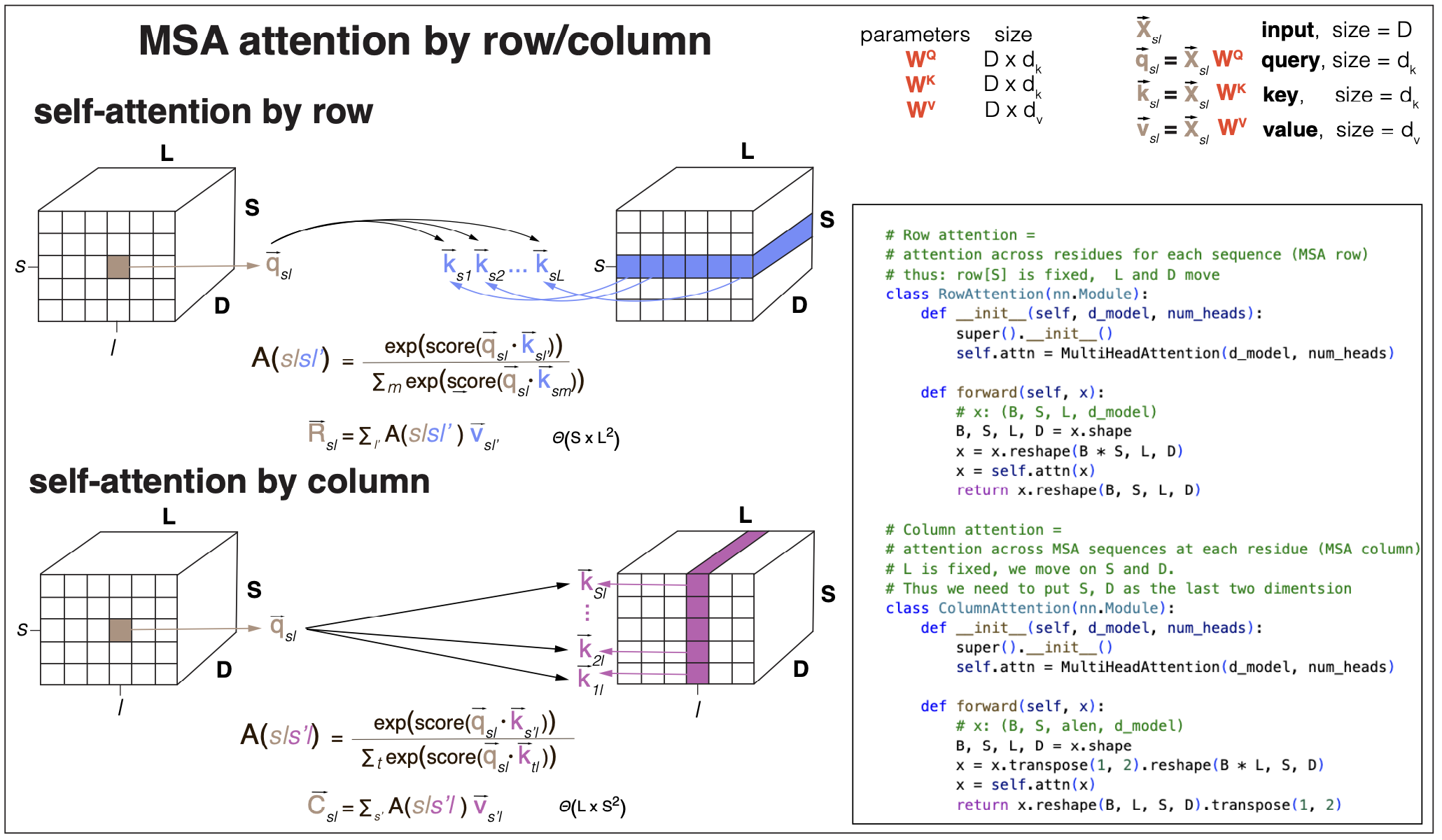
Figure 6. self-attention by row and by column (Rao et al., 2021) are examples of axial attention (Ho et al., 2019).
MSA self-attention
Given an alignment of S sequences of length L, if we apply self-attention naively as described in Figures 1 and 2, just an extension from sequences, then the time complexity to calculate the self-attention maps will scale with \((SxL)^2\) both in time and memory requirements. The time complexity is really too large for any practical purpose, and the memory required to store the attention maps would be prohibitive. For that reason, the method “MSA Transformer” by Rao et al., 2021, uses a form of attention called axial attention first introduce in the paper “Axial Attention in multidimensional transformers” by Ho et al., 2019.
Axial attention restricts in some form the number of keys that a given query attends to. For the case of input alignments, there are two obvious choices of axial attention, see Figure 6.
- Attention by row (or sequence) where queries in one sequence \(s\) attend only to keys in the same sequence. Intuitively, MSA attention by row should capture structural information contained in the alignment. The time and space requirements of attention by row scale with \(SxL^2\).
- Attention by column (or alignment position) where queries in one position \(l\) attend only to keys in the same position for all sequences. Intuitively, MSA attention by column should capture species-specific information contained in the alignment. The time and space requirements of attention by column scale with \(S^2xL\).
MSA row- and column- attention maps storage can be further reduced by tying the contributions of all rows and all columns respectively
-
Tied row attention In row attention, the contributions of all rows (sequences) can be averaged, which results in \(LxL\) tied-row attention maps.
\[TA^R[L,L] = \mbox{softmax}_K \frac{\sum_s Q^R_s[L,d_k] * (K^R)^T_s[d_k,L]}{S\sqrt{d_k}}.\]Tying row-attention makes sense for biological MSA of homologous sequences because it implies that all homologous sequences in the alignment share the structure, and contribute similarly to it.
-
Tied column attention In column attention, the contributions of all columns (positions) can be averaged, which results in \(SxS\) tied-column attention maps.
\[TA^C[S,S] = \mbox{softmax}_K \frac{\sum_l Q^C_l[S,d_k] * (K^C)^T_l[d_k,S]}{L\sqrt{d_k}}.\]Tying column-attention makes sense for biological MSA of homologous sequences because it implies that all positions in the molecule contribute similarly to estimate the relationship btw the different species represented by the sequences.
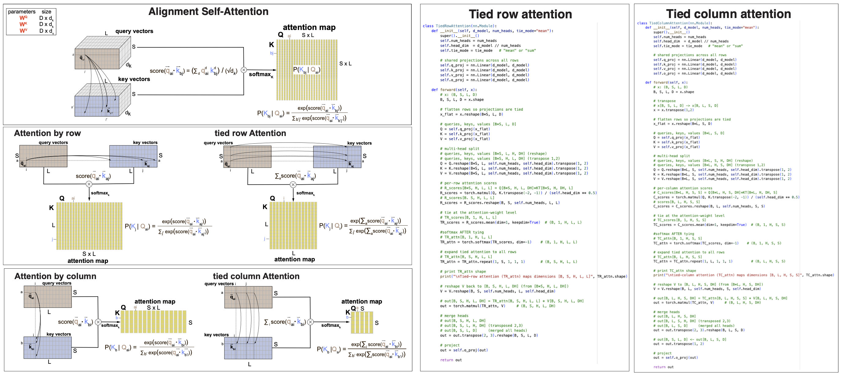
Figure 7. (A) self-attention by row and by column, untied and tied. (B) Pytorch code for the tied-column vs tied-row MSA attention mechanisms.
Figure 7A shows a comparison of the different MSA attention mechanisms discussed. Figure &B shows a line-by-line comparison between tied-row and tied-column self-attention. The actual code can be found in b3_transformer.ipynb.
Figure 8.
MSA transformer layer
The Rao et al., “MSA Transformer” is described in Figure 8.
The input is an MSA embedding of dimensions [S,L,D], where S is the number of sequences, L is the length of the alignment, and D the embedding dimension. The output is another embedding alignment of the same size. The MSA transformer alternates a row and column self-attention blocks. The attention blocks are preceded by a LayerNorm, and each forms a residual block where the inputs are added to the outputs. Final there is another residual block that processes a final fully connected network.
The output is a new MSA embedding which has learned the interactions between the query and key embeddings. These output can be used for a variety of downstream tasks. We will describe how these transformer models are trained and used for many other tasks in our next block 4 on Large language Models.
AlphaFold2: accurate protein folding with transformers
AlphaFold2 is a method based on transformers that taking a protein sequence as input predicts its 3D structure.
The paper that describes the method is this, “Highly accurate protein structure prediction with AlphaFold”, and important to actually understand all the many details of the model is the AF2 supplement. I also followed and found useful this AF2 explained blog.
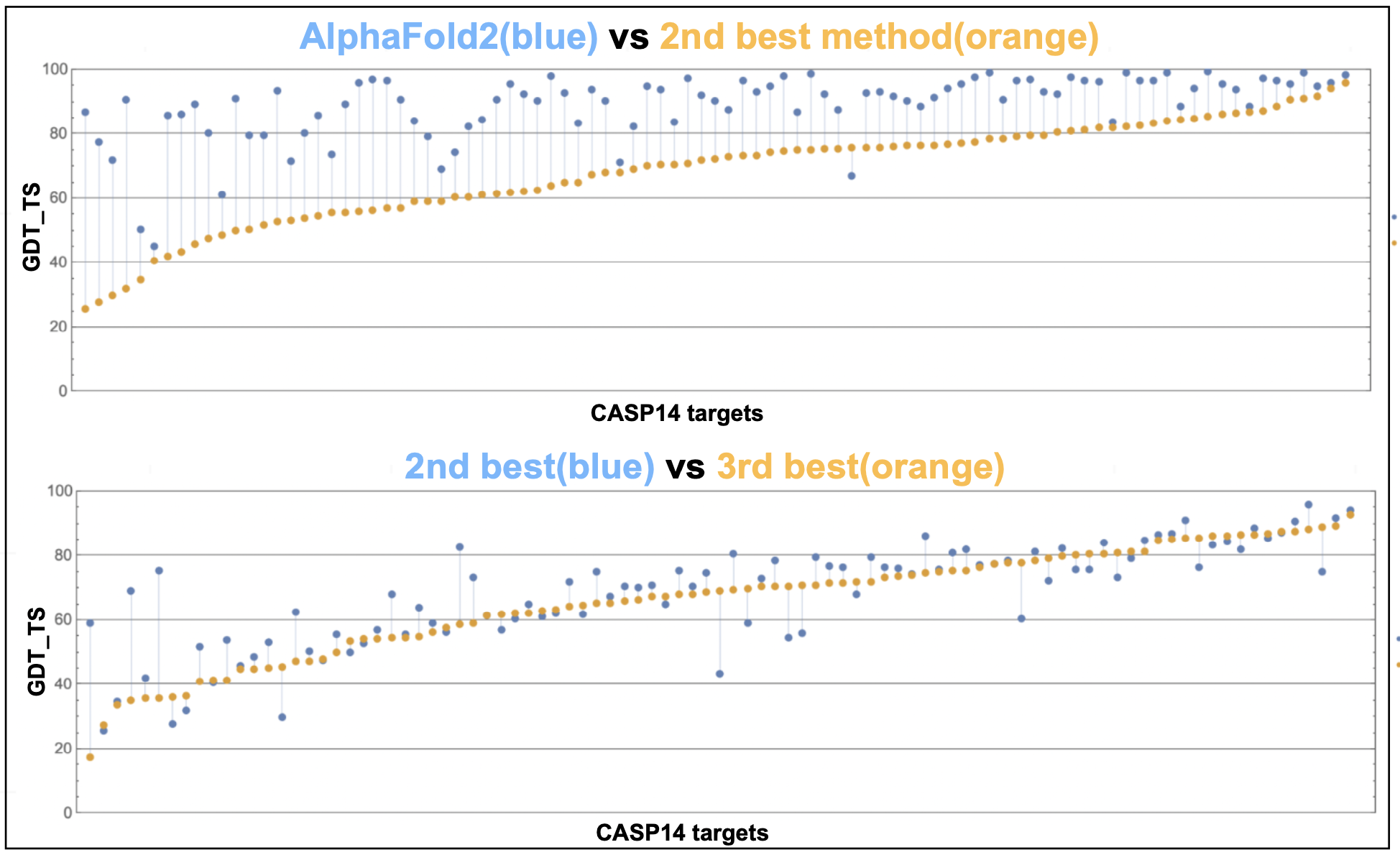
Figure 9. AlphaFold2 performance on the CASP14 target protein structures.
Highly accurate predictions!
The performance of AlphaFold2 at the CASP14 blind competition was really spectacular. There are many figures in the CASP14 paper. Perhaps for me, the one that I like more striking is this one reproduced from M. Alquraishi blog. x-axis are the different targets and y-axis is the GDT_TS (global distance test, total score) measure (ranges from 0 to 100 where higher better; above 95% is considered experimental accuracy). We can compare the difference in performance between AlphaFold2 and the second best group, with that of the second and third groups.
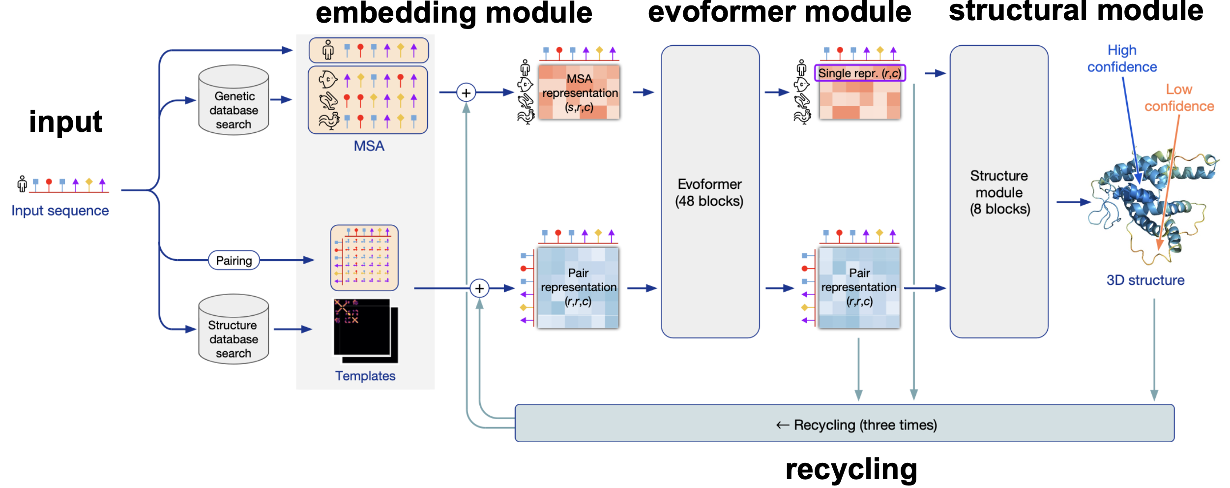
Figure 10. AlphaFold2 overview from Jumper et al. 2021.
Figure 10 is an overview of the AlphaFold2 method. It can be divided into four different blocks: the Embedding module, the Evoformer module, the Structural module, and finally recycling.
Inputs/Outputs
The input is just a protein sequence in inference mode or a mmcif file in training mode. An mmcif file includes all the information of the crystal structure of a protein, in particular it includes the sequence, and the x,y,z coordinates of all the heavy atoms. The xyz are used as labels in training to compute one of the loses.
Given the input sequence, standard databases of genomic sequences are searched with different homology methods to create an MSA. In the MSA, the first sequence is the input sequence, and the length of the MSA is the same as the length of the sequence.
The Embedding module
The primary sequence (of length r), and the alignment (of length r with s sequences) are transformed into
-
a pair representation \(z[r,r,c_z]\) for \(c_z = 128\)
-
a MSA representation \(m[s,r,c_m]\) for \(c_m = 256\).
The embedding module is described in Figure 11. Figure 11 concentrates on the description of the embedding of the sequence and the MSA into the pair and MSA representations. For more information about how to add templates and the extra MSAs please refer to the AF2 supplement.
The pair and MSA representation are the inputs of the evoformer module.
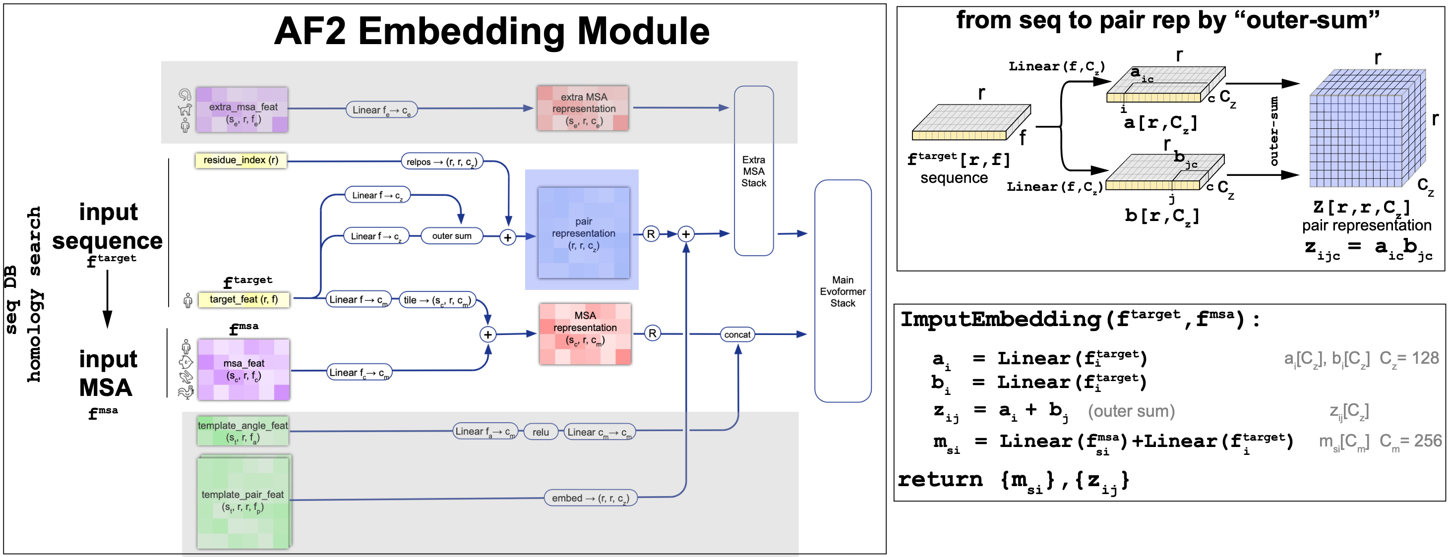
Figure 11. AlphaFold2 embedding for the initial representations. Detail of the outer-sum mechanism to generate the pair representations from the input sequences.
The Evoformer module
The Evoformer takes a pair representation \(z[r,r,c_z]\) and a MSA representation \(m[s,r,c_m]\) and returns updated versions of both representations. The main block of the evoformer that we will describe later is repeated 48 times (without sharing weights) before reporting the pair and MSA output representations.
The Evoformer (Figure 12) performs a series of MSA self-attention mechanics in the MSA track, as well new attention mechanisms on the pair representation stack (triangular attention), that we describe next. Moreover the two representations also talk to each other during the process.
The MSA stack
The MSA stack includes alternative row-wise and column-wise self-attention mechanism similar to the ones discussed earlier in this block.
-
MSA row-wise gated self-attention with pair bias. AF2 adds a contribution of the pair representation as a bias to the query/keys product, before the softmax calculation. (See Figure 12). It also adds gating, which means that an extra sigmoid (or linear logistic) MSA projection is added after to the attention maps after the softmax calculation.
-
MSA column-wise gated self-attention. The column-wise MSA attention mechanics also adds a gate at the end. This is similar to the gating that we discussed earlier with the LSTM RNNs. The effect of gating on attention is common but it’s effect on performance has only been rarely examined (here is a recent work on gating performance on transformers.
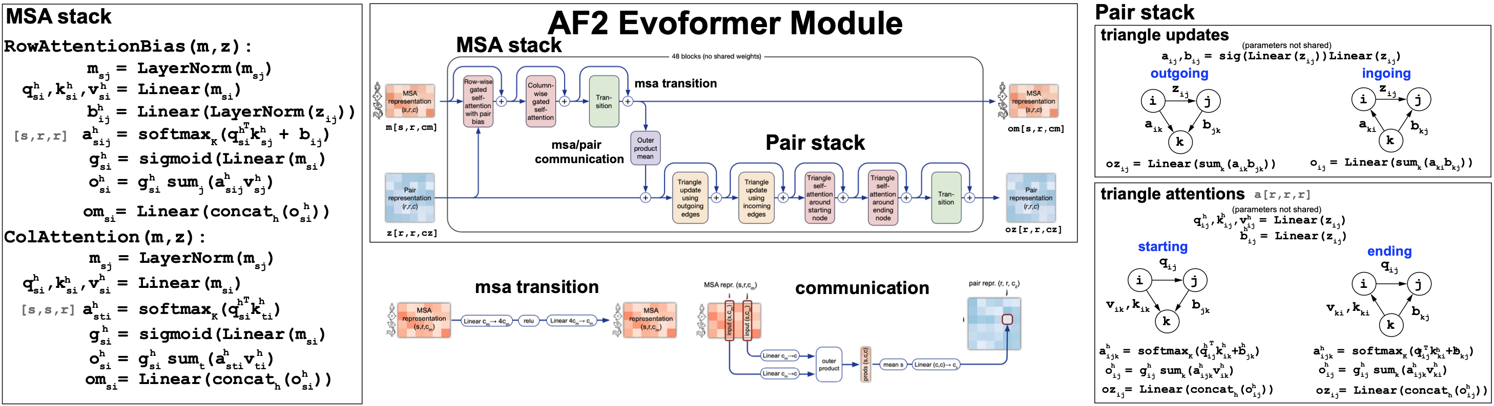
Figure 12. The AlphaFold2's Evoformer module.
The Pair stack
In the Pair stack, the pair representation embeddings are updated. It uses two different mechanisms, both described in Figure 12. Both mechanisms apply to three different positions, i, j, k, and the triangle formed by them.
-
Triangular updates. Linear projections are applied to the pair representation along the edges of the triangle. There are two symmetric versions of it.
-
Triangular attention. An attention mechanism is devised also acting between three positions, and it builds queries and keys from the different edges in the triangle. This attention mechanism also has two symmetric versions and it also includes a bias term and gating.
Communication btw the two stacks
-
The pair representation is added to the MSA stack as a bias to the row-wise attention.
-
The pair stack is update by an MSA outer-product transformation into a pair representation that is described in Figure 12.
The structural module
The inputs to the structural module both come directly from the evoformer, and they are
-
The first sequence embedding from the evoformer output MSA embedding,
-
The whole pair representation embedding form the evoformer output.
-
A geometric representation of each residue characterized by a rotation \(R\) and a translation \(t\) wrt a global frame. At initialization, all residues are located at the same arbitrary origin point.
How AF2 characterizes an amino acid: The backbone frame and torsion angles
Each amino acid in a peptide chain is a collection of many atoms that have a particular configuration. Each of the 20 different naturally occurring amino acids has a stereotyped configuration of 3 atoms: a carbon (C), a nitrogen (N) and \(\alpha\)-Carbon (\(C_{\alpha}\)), referred to as the backbone. What distinguishes one amino acid from another is the side-chain (R in Figure 13).
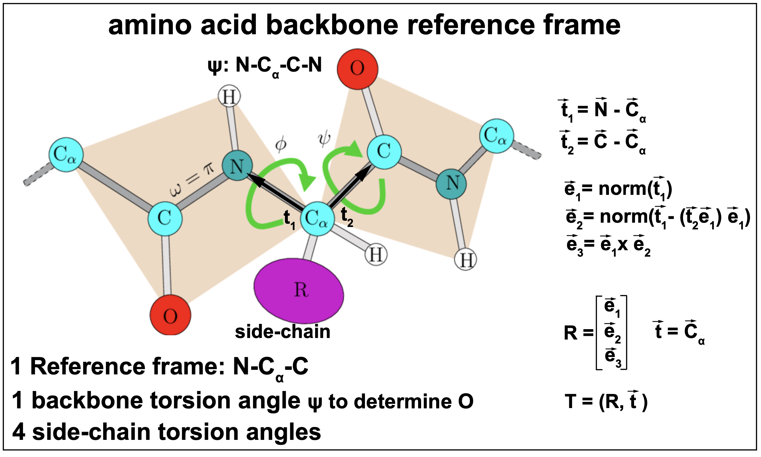
Figure 13. The amino acid backbone reference frame and torsion angles.
As described in Figure 13, AF2 characterizes each amino acid by a reference frame that puts the three atoms: N, C, and \(C_{\alpha}\) in a plane with \(C_{\alpha}\) at the origin. In the structural module, AF2 first determines the reference frame that gives us the position of the N, C, \(C_{\alpha}\), and subsequently trains torsion angles, that given the backbone frame, allows to determine all the rest of the atoms.
Each amino acid is then characterized by a rotation which is a matrix \(R[3,3]\), and a translation \(\bar{t}[3]\) that describe the 3D locations for the backbone \(C_{\alpha}\), C and N atoms. Together they are referred to as a Euclidean transformation.
Given \(T_i\) the reference frame for amino acid \(i\) in the target peptide,
\[T_i = (R_i, \bar t_i),\]and an atom with coordinates \(\bar{x}\) in the \(T_i\) reference frame, then its global coordinates \(\bar{x}_{global}\) are given by
\[\bar{x}_{global} = T_i \bar{x} =: R_i \bar{x} + \bar{t}_i.\]Moreover, for an atom with coordinates \(\bar{x}_{global}\) in the global reference frame, its coordinates in the \(T_i\) reference frame are given by
\[\bar{x} = T^{-1}_i \bar{x}_{global} = R^{-1}_i\left(\bar{x}_{global} - \bar{t}_i\right).\]The structural module outputs
The structural module’s output is the collection of all \(\{T_i\}\) transformations and torsion angles that would place the \(r\) amino acids in the target molecule in their corresponding 3D location in the structure. In order to do that, it used an attention mechanism with a novel geometric component named Invariant point attention (IPA).
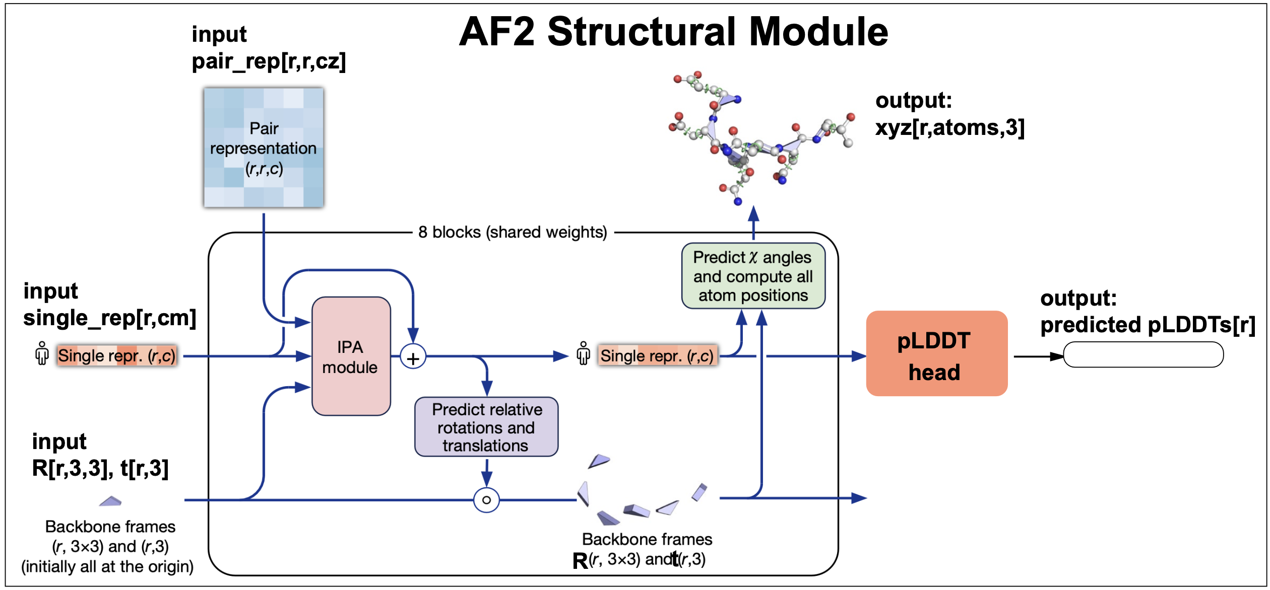
Figure 14. The AlphaFold2's structural module.
Invariant Point Attention (IPA)
IPA is a geometry-aware attention mechanism used by the structure module. All three inputs: the reference seq embedding, the pair representation and the geometric representation are included into the attention score.
Importantly, the geometric component of the attention is invariant under a global Euclidean transformation, thus the name invariant point attention.
predicted accuracy (plDDT).
Local distance difference test lDDT is a method for estimating the quality of protein structure prediction compared to a reference structure. LDDT provides a score per residue and ranges from 0 to 1. LDDT does not require an alignment of the two structures being compared, and it takes into account the distances between all the atoms in the molecule.
The AF2 structural model has a final layer that taking as input the sequence representation, it produces an output trained to predict the lDDT of the AF2 output structure, named the predicted lDDT (plDDT).
Training
Training is performed end-to-end, which means that given the sequence inputs, a forward pass through the model produces the output: MSA embedding, pair embedding, and all atom coordinates. Then, using loss functions that estimate how different those predictions are from the “true” values, the backward pass does gradient descent to update all the parameters. All parameters are changed by a quantity that is proportional to the negative value of the gradient of the loss at the current parameter values. The process repeats until the losses become small and do not change. AF2 uses Adam optimization (a particular and commonly used gradient descent implementation), and a learning rate (the proportionality constant for the gradient descent term) of \(10^{-3}\).
Losses
The network is trained end-to-end, that is, all modules are optimized at the same time. In consequence, the loss function is a combination of several different losses each guiding the different aspects of the method in training. The coefficients in front of every loss are completely empirical and determined by trial and error. Parameters that are not trained with the rest of the model are usually referred to as meta parameters.
Below, we describe some of the more significantive loss functions used in AF2.
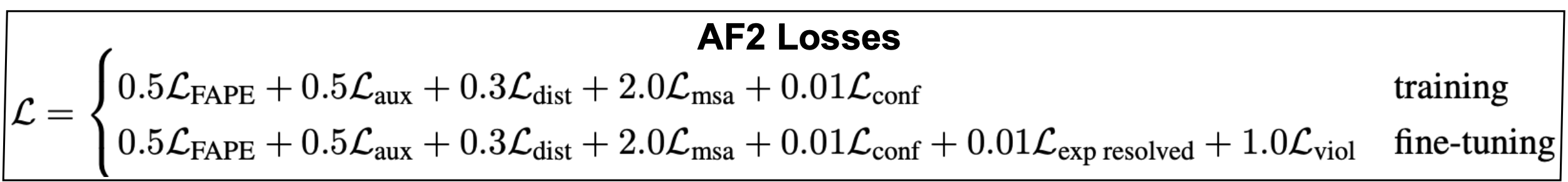
Figure 15. The AlphaFold2 losses.
-
The FAPE loss: The frame aligned point error (FAPE) is a geometric loss that takes a set of predicted positions \(\{\bar{x}_i\}\) and a set of predicted frames \(\{T_i\}\), and for any pair of positions (i,j), it calculates the relative coordinates of position \(j\) (with global precited coordinates \(\bar{x}_j\)) in the reference frame of position \(i\) (\(T_i\)) as
\[\bar{x}_{ij} =: T^{-1}_i \bar{x}_j = R_i^{-1} \left(\bar{x}_j - \bar{t}_i\right).\]\(\bar{x}_{ij}\) are the relative coordinates of residue j wrt the reference system of residue i. These predicted frame alignmed point errors (FAPE) are compared to the equivalent errors calculated using the “true” values \(\bar{x}_j^{true}\) and \(\bar{T}_i^{true}\).
AF2 calculates the distances,
\[d_{ij} = \sqrt{ || \bar{x}_{ij} - \bar{x}^{true}_{ij} ||^2 + \epsilon },\]the small value \(\epsilon > 0\) prevents the distance from becoming zero.
The \(L_{FAPE}\) is an average over (i,j) of those \(d_{ij}\) distances,
\[L_{FAPE} = \frac{1}{Z} \mbox{mean}_{ij}\left( \mbox{min}(d_{ij},d_{clamp})\right),\]where \(Z = d_{clamp} = 10\) amstrongs.
-
The distogram (dist) loss. The distogram loss The final pair-representation is symmetrized \(z_{ij}+z_{ji}\) and linearly projected, binned intro 64 bins covering between 2-22 amnstrong, and converted into a probability by softmax, \(p_{ij}[64]\). Those distributions are referred to as distograms.
The distogram loss is a supervised loss. The actual distances between amino-acids are obtained from the mmCIF files that describe the crystal structures of the proteins used in training. Those label distances and one-hot distributed in the same 64 bin structure, \(y_{ij}[64]\).
The distogram loss calculates the cross-entropy between the two as
\[L_{dist} = - \frac{1}{r^2} \sum_{i,j}\sum_{b=1}^{64} y_{ij}(b)\, \log(p_{ij}(b)).\] -
The MSA loss: The MSA loss is self-supervised. The final MSA representation is used to to reconstruct MSA values that have been previously masked out.
The MSA representation \(m_{sic}\) is projected to a \(23\) representation (20 aa + unknow + gap + mask), and softmasked into \(p_{sj}[23]\). The ground truth \(y_{si}[23]\) are one-hot encoded.
The MSA loss calculates the cross-entropy between the two as
\[L_{MSA} = - \frac{1}{N_{mask}} \sum_{s,i\in \mbox{mask}}\sum_{c=1}^{23} y_{si}(c)\, \log(p_{si}(c)).\] -
The lDDT loss. The lDDT scores of the predicted 3D structure are discretized into 50 bins and softmaxed. Those predicted lDDT scores are compared to the lDDT scores of the true structure which are one-hot encoded into 50 bins. Similarly to the previous cases, the cross entropy is calculated as the lDDT loss.
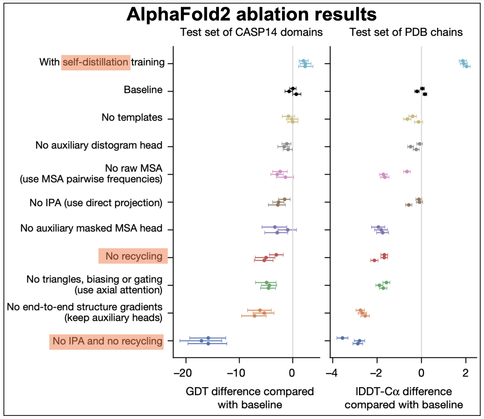
Figure 16. AF2 ablation results.
self-distillation
During the course of the AF2 implementation, it was observed that performance improved significantly by using predicted structures into the training. A method named self-distillation.
Self-distillation uses a model trained only on sequences with known 3D structures to predict the structures of many other sequences (around 350,000 diverse sequences from Uniclust3036). Then, they made a new dataset with a subset of those structures predicted with high confidence by the model (as determined by th eplDDT scores). The same model architecture was then trained on this new dataset including just predicted structures. It appears that performance significantly increases using self-distillation, as described in Figure 16.
I personally, cannot stop tinking that sefl-distillation has to be very prone to overfitting. It would be interesting to design experiment to test that.
Recycling
The whole network is executed sequentially Ncycle times, where the outputs of the former pass are recycled as inputs for the next cycle. This seems to be an important step to achieve high performance, as described in Figure 16.
In Summary
In Figure 17, I have adapted the summary figure from the original AF2 blog with some of the features we have discussed in this lectures.
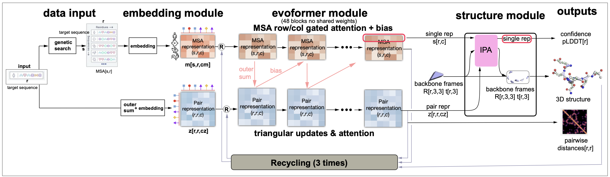
Figure 17. The AlphaFold2 summary.
Some important characteristics of AlphaFold2 are
-
Directly predicts the 3D coordinates of all heavy atoms for a given protein from the amino acid sequence using aligned sequences of homologs as inputs.
-
Uses alignments and pair representations with different attention mechanisms for each of them, but treated jointly such that they exchange information with each other. For a protein sequence of length L, it builds SxL alignments and constructs LxL maps (called pair representations) to describe connections between the different positions.
-
The method is trained end-to-end, that is all parameters are updated in the one single gradient descent optimization routine
-
Uses many different loss functions some used at intermediate stages, and a final global loss function used to optimize all parameters of the model at once.
-
Used a method called self-distillation to learn from unlabeled proteins. Self-distillation uses predictions of the model for further training.
-
It is able to estimate accuracy
-
Introduces a new formalism for protein 3D structure prediction by providing a rotation and translation to identify the location of each amino acid in a protein molecule. All residues are trivially initialized at the same location which evolves with training into an accurate description of all atoms of the amino acid chain.